JEE Main & Advanced

This is the most popular co-ordinate system.   Axis of \[x\] : The line \[XOX'\] is called axis of \[x\].   Axis of \[y\] : The line \[YOY'\] is called axis of \[y\].   Co-ordinate axes : \[x\] axis and \[y\] axis together are called axis of  co-ordinates or axes of reference.   Origin : The point \['O'\] is called the origin of co-ordinates or the origin.   Let \[OL=x\] and \[OM=y\] which are respectively called the abscissa (or x-coordinate) and the ordinate (or y-coordinate). The       co-ordinate of P are \[(x,\,\,y)\].     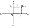Here, co-ordinates of the origin is (0, 0). The y co-ordinates of every point on x-axis is zero.   The x co-ordinates of every point on y-axis is zero.   Oblique axes : If both the axes are not perpendicular then they are more...

Co-ordinates of a point are the real variables associated in an order to a point to describe its location in some space. Here the space is the two dimensional plane.     The two lines \[XOX'\] and \[YOY'\] divide the plane in four quadrants. \[XOY,\text{ }YOX',\text{ }X'OY',\text{ }Y'OX\] are respectively called the first, the second, the third and the fourth quadrants. We assume the directions of \[OX,\,OY\] as positive while the directions of \[OX',\text{ }OY'\] as negative.

(1) Geometrical method for probability : When the number of points in the sample space is infinite, it becomes difficult to apply classical definition of probability. For instance, if we are interested to find the probability that a point selected at random from the interval [1, 6] lies either in the interval [1, 2] or [5, 6], we cannot apply the classical definition of probability. In this case we define the probability as follows:     \[P\{x\in A\}=\frac{\text{Measure of region }A}{\text{Measure of the sample space }S}\]     where measure stands for length, area or volume depending upon whether S is a one-dimensional, two-dimensional or three-dimensional region.     (2) Probability distribution : Let S be a sample space. A random variable X is a function from the set S to R, the set of real numbers.     For example, the sample space for a throw of a pair more...

(1) The law of total probability : Let S be the sample space and let \[{{E}_{1}},\,{{E}_{2}},\,.....{{E}_{n}}\] be n mutually exclusive and exhaustive events associated with a random experiment. If A is any event which occurs with \[{{E}_{1}}\] or \[{{E}_{2}}\] or …or  \[{{E}_{n}},\] then     \[P(A)=P({{E}_{1}})\,P(A/{{E}_{1}})+P({{E}_{2}})\,P(A/{{E}_{2}})+...+P({{E}_{n}})\,P(A/{{E}_{n}})\].     (2) Baye’s rule : Let S be a sample space and \[{{E}_{1}},\,{{E}_{2}},\,.....{{E}_{n}}\] be n mutually exclusive events such that \[\bigcup\limits_{i=1}^{n}{{{E}_{i}}}=S\] and \[P({{E}_{i}})>0\] for \[i=\text{ }1,\text{ }2,\text{ }\ldots \ldots ,n\]. We can think of (\[{{E}_{i}}'s\] as the causes that lead to the outcome of an experiment. The probabilities \[P({{E}_{j}}),\,\,i=1,\,\,2,\,\,...,\,n\]  are called  prior probabilities. Suppose the experiment results in an outcome of event A, where \[P(A)>0\]. We have to find the probability that the observed event A was due to cause \[{{E}_{i}},\] that is, we seek the conditional probability \[P({{E}_{i}}/A)\]. These probabilities are called posterior probabilities, given by Baye’s rule as \[P({{E}_{i}}/A)=\frac{P({{E}_{i}}).P(A/{{E}_{i}})}{\sum\limits_{k=1}^{n}{P({{E}_{k}})\,P(A/{{E}_{k}})}}\].

Let A and B be two events associated with a random experiment. Then, the probability of occurrence of A under the condition that B has already occurred and \[P(B)\ne 0,\] is called the conditional probability and it is denoted by \[P(A/B)\].     Thus, \[P(A/B)=\] Probability of occurrence of A, given that B has already happened.     \[=\frac{P(A\cap B)}{P(B)}=\frac{n(A\cap B)}{n(B)}\].     Similarly, \[P(B/A)=\] Probability of occurrence of B, given that A has already happened.     \[=\frac{P(A\cap B)}{P(A)}=\frac{n(A\cap B)}{n(A)}\].    

• Sometimes, \[P(A/B)\] is also used to denote the probability of occurrence of A when B Similarly, \[P(B/A)\] is used to denote the probability of occurrence of B when A occurs.

    (1) Multiplication theorems on probability     (i) If A and B are two events associated with a random experiment, then\[P(A\cap B)=P(A)\,.\,P(B/A)\], if \[P(A)\ne 0\] or \[P(A\cap B)=P(B)\,.\,P(A/B)\], if \[P(B)\ne 0\]. more...

Notations : (i) \[P(A+B)\text{ or }P(A\cup B)=\] Probability of happening of A or B     = Probability of happening of the events A or B or both     = Probability of occurrence of at least one event A or B     (ii) \[P(AB)\] or \[P(A\cap B)=\] Probability of happening of events A and B together.     (1) When events are not mutually exclusive : If A and B are two events which are not mutually exclusive, then     \[P(A\cup B)=P(A)+P(B)-P(A\cap B)\]     or  \[P(A+B)=P(A)+P(B)-P(AB)\]     For any three events A, B, C     \[P(A\cup B\cup C)=P(A)+P(B)+P(C)-P(A\cap B)\]\[-P(B\cap C)-P(C\cap A)+P(A\cap B\cap C)\]     or \[P(A+B+C)=P(A)+P(B)+P(C)-P(AB)-P(BC)\]\[-P(CA)+P(ABC)\]     (2) When events are mutually exclusive : If A and B are mutually exclusive events, then \[n(A\cap B)=0\] \[\Rightarrow \] \[P(A\cap B)=0\]     \[\therefore \]\[P(A\cup B)=P(A)+P(B)\].     For any three events A, B, more...

As a result of an experiment if \[''a''\] of the outcomes are favourable to an event E and \[''b''\] of the outcomes are against it, then we say that odds are a to b in favour of E or odds are b to a against E.     Thus odds in favour of an event E     \[=\frac{\text{Number of favourable cases}}{\text{Number of unfavourable cases}}=\frac{a}{b}=\frac{a/(a+b)}{b/(a+b)}=\frac{P(E)}{P(\bar{E})}\].     Similarly, odds against an event E     \[=\frac{\text{Number of unfavourable cases}}{\text{Number of favourable cases}}=\frac{b}{a}=\frac{P(\bar{E})}{P(E)}\].

(1) Problems based on combination or selection : To solve such kind of problems, we use \[^{n}{{C}_{r}}=\frac{n\,!}{r!(n-r)!}\].     (2) Problems based on permutation or arrangement : To solve such kind of problems, we use \[^{n}{{P}_{r}}=\frac{n\,!}{(n-r)!}\].

If a random experiment results in n mutually exclusive, equally likely and exhaustive outcomes, out of which m are favourable to the occurrence of an event A, then the probability of occurrence of A is given by     \[P(A)=\frac{m}{n}=\frac{\text{Number of outcomes favourable to }A}{\text{Number of total outcomes}}\]     It is obvious that \[0\le m\le n\]. If an event A is certain to happen, then \[m=n,\] thus \[P(A)=1\].     If A is impossible to happen, then \[m=0\] and so \[P(A)=0\]. Hence we conclude that \[0\le P(A)\le 1\].     Further, if \[\bar{A}\] denotes negative of A i.e. event that A doesn’t happen, then for above cases m, n; we shall have      \[P(\bar{A})=\frac{n-m}{n}=1-\frac{m}{n}=1-P(A)\] ,\[\therefore \]  \[P(A)+P(\bar{A})=1\].     Notations : For two events A and B,     (i) \[A'\] or \[\bar{A}\] or \[{{A}^{C}}\] stands for the non-occurrence or negation of A.     (ii) \[A\cup B\] more...

(1) Sample space : The set of all possible outcomes of a trial (random experiment) is called its sample space. It is generally denoted by S and each outcome of the trial is said to be a sample point.     (2) Event : An event is a subset of a sample space.     (i) Simple event : An event containing only a single sample point is called an elementary or simple event.     (ii) Compound events : Events obtained by combining together two or more elementary events are known as the compound events or decomposable events.     (iii) Equally likely events : Events are equally likely if there is no reason for an event to occur in preference to any other event.     (iv) Mutually exclusive or disjoint events : Events are said to be mutually exclusive or disjoint or incompatible if the occurrence of more...