Current Affairs JEE Main & Advanced

In this section, we shall discuss how Venn diagrams are used to represent truth and falsity of statements or propositions. For this, let us consider the statement: “All teachers are scholars”. Let us assume that this statement is true. To represent the truth of the above statement, we define the following sets     \[U\]= the set of all human beings     S  = the set of all scholars     And T  = the set of all teachers     Clearly, \[S\subset U\] and \[T\subset U\]     According to the above statement , if follows that \[T\subset S\]. 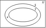Thus, the truth of the above statement can be represented by the Venn diagram shown in        Now, if we consider the statement : ? There are some scholars who are teachers?,  It is evident from the Venn diagram that there is a scholar x who is not a teacher. Therefore, the above statement is false and its truth value is ?F?. Thus,  we can also check the truth and falsity of other statements which are connected to a given statement.  

Propositions : A statement or a proposition is an assertive (or declarative) sentence which is either true or false but not both a true statement is called valid statement. If a statement is false, then it is called invalid statement.     Open statement : A declarative sentence containing variable (s) is an open statement if it becomes a statement when the variable (s) is (are) replaced by some definite value (s).     Truth Set : The set of all those values of the variable (s) in an open statement for which it becomes a true statement is called the truth set of the open statement.     Truth Value : The truth or falsity of a statement is called its truth value.     If a statement is true, then we say that its truth value is ‘True’ or ‘T’. On the other hand the truth value of a false statement is ‘False’ or ‘F’.     Logical variables : In the study of logic, statements are represented by lower case letters such as p, q, r, s.. These letters are called logical variables.     For example, the statement ‘The sun is a star’ may be represented or denoted by p and we write p : The sun is a star     Similarly, we may denote the statement \[145=\text{ }2\].     Quantifiers : The symbol \[\forall \](stands for ‘for all’) and \[\exists \](stands for “there exists”) are known as quantifiers.     In other word, quantifiers are symbols used to denote a group of words or a phrase.     The symbols \[\forall \] and \[\exists \] are known as existential quantifiers. An open sentence used with quantifiers always becomes a statement.     Quantified statements : The statements containing quantifiers are known as quantified statements.     \[{{x}^{2}}>0.\forall x\in R\] is a quantified statement. Its truth value is T.

Logic was extensively developed in Greece. In the middle ages the treatises of Aristotle concerning logic were re-discovered. The axiomatic approach to logic was first proposed by George Boole. On this account logic  relative to mathematics is sometimes called Boolean logic. It is also called mathematical logic or more recently symbolic logic.     The dictionary meaning of the word ‘Logic’ is “the science of reasoning”. It is the study and analysis of the nature of valid arguments. In the process of reasoning we communicate our ideas or thoughts with the help of sentences in a particular language. The following types of sentences are normally used in our every day communication.   (1) Assertive sentence   (2) Imperative sentence   (3) Exclamatory sentence   (4) Interrogative sentence     In this chapter, we shall be discussing about a specific type of sentences which will called as statement or propositions.

(1) Advantages : Linear programming is used to minimize the cost of production for maximum output. In short, with the help of linear programming models, a decision maker can most efficiently and effectively employ his production factor and limited resources to get maximum profit at minimum cost.   (2) Limitations  : (i) The linear programming can be applied only when the objective function and all the constraints can be expressed in terms of linear equations/inequations.   (ii) Linear programming techniques provide solutions only when all the elements related to a problem can be quantified.   (iii) The coefficients in the objective function and in the constraints must be known with certainty and should remain unchanged during the period of study.   (iv) Linear programming technique may give fractional valued answer which is not desirable in some problems.

(1) Bounded region: The region surrounded by the inequations \[ax+by\le m\] and \[cx+dy\le n\] in first quadrant is called bounded region. It is of the form of triangle or quadrilateral. Change these inequations into equations, then by putting \[x=0\] and \[y=0,\] we get the solution. Also by solving the equations we get the vertices of bounded region.     The maximum value of objective function lies at one vertex in limited region.     (2) Unbounded region : The region surrounded by the inequations \[ax+by\ge m\] and \[cx+dy\ge n\] in first quadrant, is called unbounded region.     Change the inequation in equations and solve for \[x=0\]and \[y=0\]. Thus we get the vertices of feasible region.     The minimum value of objective function lies at one vertex in unbounded region but there is no existence of maximum value.

There are two techniques of solving an L.P.P. by graphical method. These are :     (1) Corner point method          (2) Iso-profit or Iso-cost method     (1) Corner point method     Working Rule:     (i) Formulate mathematically the L.P.P.     (ii) Draw graph for every constraint.     (iii) Find the feasible solution region.     (iv) Find the coordinates of the vertices of feasible solution region.     (v) Calculate the value of objective function at these vertices.     (vi) Optimal value (minimum or maximum) is the required solution.     (vii) If there is no possibility to determine the point at which the suitable solution found, then the solution of problem is unbounded.     (viii) If feasible region is empty, then there is no solution for the problem.     (ix) Nearer to the origin, the objective function is minimum and that of further from the origin, the objective function is maximum.     (2) Iso-profit or Iso-cost method : Various steps of the method are as follows :     (i) Find the feasible region of the L.P.P.     (ii) Assign a constant value \[{{Z}_{1}}\] to Z and draw the corresponding line of the objective function.     (iii) Assign another value \[{{Z}_{2}}\] to Z and draw the corresponding line of the objective function.     (iv) If \[{{Z}_{1}}<{{Z}_{2}},({{Z}_{1}}>{{Z}_{2}})\], then in case of maximization (minimization) move the line P1Q1 corresponding to \[{{Z}_{1}}\] to the line \[{{P}_{2}}{{Q}_{2}}\] corresponding to \[{{Z}_{2}}\] parallel to itself as far as possible, until the farthest point within the feasible region is touched by this line. The coordinates of the point give maximum (minimum) value of the objective function.     (v) The problem with more equations/inequations can be handled easily by this method.     (vi) In case of unbounded region, it either finds an optimal solution or declares an unbounded solution. Unbounded solutions are not considered optimal solution. In real world problems, unlimited profit or loss is not possible.

There are mainly four steps in the mathematical formulation of a linear programming problem, as mathematical model. We will discuss formulation of those problems which involve only two variables.     (1) Identify the decision variables and assign symbols x and y to them. These decision variables are those quantities whose values we wish to determine.     (2) Identify the set of constraints and express them as linear equations/inequations in terms of the decision variables. These constraints are the given conditions.     (3) Identify the objective function and express it as a linear function of decision variables. It may take the form of maximizing profit or production or minimizing cost.     (4) Add the non-negativity restrictions on the decision variables, as in the physical problems, negative values of decision variables have no valid interpretation.

The term programming means planning and refers to a process of determining a particular program.     (1) Objective function : The linear function which is to be optimized (maximized or minimized) is called objective function of the L.P.P.     (2) Constraints or Restrictions : The conditions of the problem expressed as simultaneous equations or inequations are called constraints or restrictions.     (3) Non-negative constraints : Variables applied in the objective function of a linear programming problem are always  non-negative. The inequations which represent such constraints are called non-negative constraints.     (4) Basic variables : The \[m\] variables associated with columns of the \[m\times n\] non-singular matrix which may be different from zero, are called basic variables.     (5) Basic solution : A solution in which the vectors associated to m variables are linear and the remaining \[(n-m)\] variables are zero, is called a basic solution. A basic solution is called a degenerate basic solution, if at least one of the basic variables is zero and basic solution is called non-degenerate, if none of the basic variables is zero.     (6) Feasible solution : The set of values of the variables which satisfies the set of constraints of linear programming problem (L.P.P) is called a feasible solution of the L.P.P.     (7) Optimal solution : A feasible solution for which the objective function is minimum or maximum is called optimal solution.     (8) Iso-profit line : The line drawn in geometrical area of feasible region of L.P.P. for which the objective function (to be maximized) remains constant at all the points lying on the line, is called iso-profit line.     If the objective function is to be minimized then these lines are called iso-cost lines.     (9) Convex set : In linear programming problems feasible solution is generally a polygon in first quadrant. This polygon is convex. It means if two points of polygon are connected by a line, then the line must be inside the polygon. 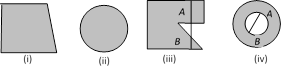For example,   (i) and (ii) are convex set while (iii) and (iv) are not convex set.

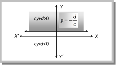
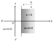
(1) Graph of linear inequations     (i) Linear inequation in one variable: \[ax+b>0,\] \[ax+b<0,\]\[cy+d>0\] etc. are called linear inequations in one variable. Graph of these inequations can be drawn as follows :     The graph of \[ax+b>0\] and \[ax+b<0\] are obtained by dividing xy-plane in two semi-planes by the line \[x=-\frac{b}{a}\](which is parallel to y-axis). Similarly for \[cy+d>0\]and \[cy+d<0\].       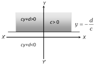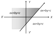(ii) Linear Inequation in two variables : General form of these inequations are \[ax+by>c,ax+by<c\]. If any ordered pair \[\left( {{x}_{1}},{{y}_{1}} \right)\] satisfies an inequation, then it is said to be a solution of the inequation.   The graph of these inequations is given below (for \[c>0\]) :   Working Rule : To draw the graph of an inequation, following procedure is followed :     (i) Write the equation \[ax+by=c\] in place of \[ax+by<c\] and \[ax+by>c\].     (ii) Make a table for the solutions of \[ax+by=c\].     (iii) Now draw a line with the help of these points. This is the graph of the line \[ax+by=c\].     (iv) If the inequation is > or <, then the points lying on this line is not considered and line is drawn dotted or discontinuous.     (v) If the ineuqation is \[\ge \] or\[\le \], then the points lying on the line is considered and line is drawn bold or continuous.     (vi) This line divides the plane XOY in two region.     To Find the region that satisfies the inequation, we apply the following rules:     (a) Take an arbitrary point which will be in either region.     (b) If it satisfies the given inequation, then the required region will be the region in which the arbitrary point is  located.     (c) If it does not satisfy the inequation, then the other region is the required region.     (d) Draw the lines in the required region or make it shaded.     (2) Simultaneous linear inequations in two variables : Since the solution set of a system of simultaneous linear inequations is the set of all points in two dimensional space which satisfy all the inequations simultaneously. Therefore to find the solution set we find the region of the plane common to all the portions comprising the solution set of given inequations. In case there is no region common to all the solutions of the given inequations, we say that the solution set is void or empty.     (3) Feasible region  : The limited (bounded) region of the graph made by two inequations is called feasible region. All the points in feasible region constitute the solution of a system of inequations. The feasible more...

(1) \[2{{\sin }^{-1}}x={{\sin }^{-1}}(2x\sqrt{1-{{x}^{2}}})\],                If \[-\frac{1}{\sqrt{2}}\le x\le \frac{1}{\sqrt{2}}\]\[\]     (2) \[2{{\sin }^{-1}}x=\pi -{{\sin }^{-1}}2x\sqrt{1-{{x}^{2}}}\],          If \[\frac{1}{\sqrt{2}}\le x\le 1\]     (3) \[2{{\sin }^{-1}}x=-\pi -{{\sin }^{-1}}(2x\sqrt{1-{{x}^{2}})}\],     If \[-1\le x\le \frac{-1}{\sqrt{2}}\]     (4) \[3{{\sin }^{-1}}x={{\sin }^{-1}}(3x-4{{x}^{3}}),\]                        If \[\frac{-1}{2}\le x\le \frac{1}{2}\]     (5) \[3{{\sin }^{-1}}x=\pi -{{\sin }^{-1}}(3x-4{{x}^{3}})\],                  If \[\frac{1}{2}<x\le 1\]     (6) \[3{{\sin }^{-1}}x=-\pi -{{\sin }^{-1}}(3x-4{{x}^{3}}),\]                If \[-1\le x<-\frac{1}{2}\]     (7) \[2{{\cos }^{-1}}x={{\cos }^{-1}}(2{{x}^{2}}-1)\],                         If \[0\le x\le 1\]     (8) \[2{{\cos }^{-1}}x=2\pi -{{\cos }^{-1}}(2{{x}^{2}}-1)\],                                If \[-1\le x\le 0\]     (9) \[3{{\cos }^{-1}}x={{\cos }^{-1}}(4{{x}^{3}}-3x)\],                       If \[\frac{1}{2}\le x\le 1\]     (10) \[3{{\cos }^{-1}}x=2\pi -{{\cos }^{-1}}(4{{x}^{3}}-3x),\]            If \[-\frac{1}{2}\le x\le \frac{1}{2}\]     (11)  \[3{{\cos }^{-1}}x=2\pi +{{\cos }^{-1}}(4{{x}^{3}}-3x),\]         If \[-1\le x\le -\frac{1}{2}\]     (12)  \[2{{\tan }^{-1}}x={{\tan }^{-1}}\left( \frac{2x}{1-{{x}^{2}}} \right)\],                     If \[-1<x\le 1\]     (13)  \[2{{\tan }^{-1}}x=\pi +{{\tan }^{-1}}\left( \frac{2x}{1-{{x}^{2}}} \right)\] ,                           If \[x>1\]     (14) \[2{{\tan }^{-1}}x=-\pi +{{\tan }^{-1}}\left( \frac{2x}{1-{{x}^{2}}} \right)\],                            If \[x<-1\]     (15) \[2{{\tan }^{-1}}x={{\sin }^{-1}}\left( \frac{2x}{1+{{x}^{2}}} \right)\] ,                   If \[-1\le x\le 1\]     (16) \[2{{\tan }^{-1}}x=\pi -{{\sin }^{-1}}\left( \frac{2x}{1+{{x}^{2}}} \right)\] ,                            If \[x>1\]     (17) \[2{{\tan }^{-1}}x=-\pi -{{\sin }^{-1}}\left( \frac{2x}{1+{{x}^{2}}} \right)\] ,                           If \[x<-1\]     (18) \[2{{\tan }^{-1}}x={{\cos }^{-1}}\left( \frac{1-{{x}^{2}}}{1+{{x}^{2}}} \right)\],                                If \[0\le x<\infty \]     (19) \[2{{\tan }^{-1}}x=-{{\cos }^{-1}}\left( \frac{1-{{x}^{2}}}{1+{{x}^{2}}} \right)\] ,                             If \[-\infty <x\le 0\]     (20) \[3{{\tan }^{-1}}x={{\tan }^{-1}}\left( \frac{3x-{{x}^{3}}}{1-3{{x}^{2}}} \right)\],                              If \[\frac{-1}{\sqrt{3}}<x<\frac{1}{\sqrt{3}}\]     (21) \[3{{\tan }^{-1}}x=\pi +{{\tan }^{-1}}\left( \frac{3x-{{x}^{3}}}{1-3{{x}^{2}}} \right)\] ,    If \[x>\frac{1}{\sqrt{3}}\]     (22) \[3{{\tan }^{-1}}x=-\pi +{{\tan }^{-1}}\left( \frac{3x-{{x}^{3}}}{1-3{{x}^{2}}} \right)\] ,   If \[x<-\frac{1}{\sqrt{3}}\]     (23)  \[{{\tan }^{-1}}\left[ \frac{x}{\sqrt{{{a}^{2}}-{{x}^{2}}}} \right]={{\sin }^{-1}}\frac{x}{a}\]                (24) \[{{\tan }^{-1}}\left[ \frac{3{{a}^{2}}x-{{x}^{3}}}{a({{a}^{2}}-3{{x}^{2}})} \right]=3{{\tan }^{-1}}\frac{x}{a}\]     (25) \[{{\tan }^{-1}}\left[ \frac{\sqrt{1+{{x}^{2}}}+\sqrt{1-{{x}^{2}}}}{\sqrt{1+{{x}^{2}}}-\sqrt{1-{{x}^{2}}}} \right]=\frac{\pi }{4}+\frac{1}{2}{{\cos }^{-1}}{{x}^{2}}\]     (26) \[{{\tan }^{-1}}\sqrt{\frac{1-x}{1+x}}=\frac{1}{2}{{\cos }^{-1}}x\]