 If we say that P is the point \[\mathbf{r}\], then we mean that the position vector of \[P\] is \[\mathbf{r}\] with respect to some origin \[O\].
(1) \[\overrightarrow{AB}\] in terms of the position vectors of points A and B : If \[\mathbf{a}\] and b are position vectors of points A and B respectively. Then, \[\overrightarrow{OA}=\mathbf{a},\,\overrightarrow{OB}=\mathbf{b}\]
\[\therefore \] \[\overrightarrow{AB}\] = (Position vector of B) – (Position vector of A)
\[=\overrightarrow{OB}-\overrightarrow{OA}=\mathbf{b}-\mathbf{a}\]
(2) Position vector of a dividing point : The position vectors of the points dividing the line \[AB\]in the ratio m : n internally or externally are \[\frac{m\mathbf{b}+n\mathbf{a}}{m+n}\] or \[\frac{m\mathbf{b}-n\mathbf{a}}{m-n}\].
If we say that P is the point \[\mathbf{r}\], then we mean that the position vector of \[P\] is \[\mathbf{r}\] with respect to some origin \[O\].
(1) \[\overrightarrow{AB}\] in terms of the position vectors of points A and B : If \[\mathbf{a}\] and b are position vectors of points A and B respectively. Then, \[\overrightarrow{OA}=\mathbf{a},\,\overrightarrow{OB}=\mathbf{b}\]
\[\therefore \] \[\overrightarrow{AB}\] = (Position vector of B) – (Position vector of A)
\[=\overrightarrow{OB}-\overrightarrow{OA}=\mathbf{b}-\mathbf{a}\]
(2) Position vector of a dividing point : The position vectors of the points dividing the line \[AB\]in the ratio m : n internally or externally are \[\frac{m\mathbf{b}+n\mathbf{a}}{m+n}\] or \[\frac{m\mathbf{b}-n\mathbf{a}}{m-n}\].
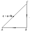 (ii) Parallelogram law of addition : If in a parallelogram \[OACB,\] \[\overrightarrow{OA}=\mathbf{a},\,\overrightarrow{OB}=\mathbf{b}\] and \[\overrightarrow{OC}\,=\mathbf{c}\]
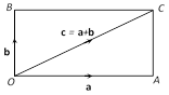 Then \[\overrightarrow{OA}+\overrightarrow{OB}=\overrightarrow{OC}\] i.e., \[\mathbf{a}+\mathbf{b}=\mathbf{c}\ \], where OC is a diagonal of the parallelogram OABC.
(iii) Addition in component form : If the vectors are defined in terms of \[\mathbf{i,}\,\,\,\mathbf{j}\] and \[\mathbf{k,}\] i.e., if \[\mathbf{a}={{a}_{1}}\mathbf{i}+{{a}_{2}}\mathbf{j}+{{a}_{3}}\mathbf{k}\] and \[\mathbf{b}={{b}_{1}}\mathbf{i}+{{b}_{2}}\mathbf{j}+{{b}_{3}}\mathbf{k}\], then their sum is defined as \[\mathbf{a}+\mathbf{b}=({{a}_{1}}+{{b}_{1}})\mathbf{i}+({{a}_{2}}+{{b}_{2}})\mathbf{j}+({{a}_{3}}+{{b}_{3}})\mathbf{k}\].
Properties of vector addition : Vector addition has the following properties.
(a) Binary operation : The sum of two vectors is always a vector.
(b) Commutativity : For any two vectors \[\mathbf{a}\] and \[\mathbf{b}\], \[\mathbf{a}+\mathbf{b}=\mathbf{b}+\mathbf{a}\].
(c) Associativity : For any three vectors \[\mathbf{a},\,\mathbf{b}\] and \[\mathbf{c}\], \[\mathbf{a}+(\mathbf{b}+\mathbf{c})=(\mathbf{a}+\mathbf{b})+\mathbf{c}\].
(d) Identity : Zero vector is the identity for addition. For any vector \[\mathbf{a},\,\,\mathbf{0}+\mathbf{a}=\mathbf{a}=\mathbf{a}+\mathbf{0}\]
(e) Additive inverse : For every vector \[\mathbf{a}\] its negative vector \[-\mathbf{a}\] exists such that \[\mathbf{a}+(-\mathbf{a})=(-\mathbf{a})+\mathbf{a}=\mathbf{0}\] i.e., \[(-\mathbf{a})\] is the additive inverse of the vector \[\mathbf{a}\].
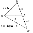
(2) Subtraction of vectors : If \[\mathbf{a}\]and \[\mathbf{b}\] are two vectors, then their subtraction \[\mathbf{a}-\mathbf{b}\] is defined as\[\mathbf{a}-\mathbf{b}=\mathbf{a}+(-\mathbf{b})\] where \[-\mathbf{b}\] is the negative of \[\mathbf{b}\] having magnitude equal to that of \[\mathbf{b}\] and direction opposite to \[\mathbf{b}\]. If \[\mathbf{a}={{a}_{1}}\mathbf{i}+{{a}_{2}}\mathbf{j}+{{a}_{3}}\mathbf{k}\], \[\mathbf{b}={{b}_{1}}\mathbf{i}+{{b}_{2}}\mathbf{j}+{{b}_{3}}\mathbf{k}\]
Then \[\mathbf{a}-\mathbf{b}=({{a}_{1}}-{{b}_{1}})\mathbf{i}+({{a}_{2}}-{{b}_{2}})\mathbf{j}+({{a}_{3}}-{{b}_{3}})\mathbf{k}\].
Then \[\overrightarrow{OA}+\overrightarrow{OB}=\overrightarrow{OC}\] i.e., \[\mathbf{a}+\mathbf{b}=\mathbf{c}\ \], where OC is a diagonal of the parallelogram OABC.
(iii) Addition in component form : If the vectors are defined in terms of \[\mathbf{i,}\,\,\,\mathbf{j}\] and \[\mathbf{k,}\] i.e., if \[\mathbf{a}={{a}_{1}}\mathbf{i}+{{a}_{2}}\mathbf{j}+{{a}_{3}}\mathbf{k}\] and \[\mathbf{b}={{b}_{1}}\mathbf{i}+{{b}_{2}}\mathbf{j}+{{b}_{3}}\mathbf{k}\], then their sum is defined as \[\mathbf{a}+\mathbf{b}=({{a}_{1}}+{{b}_{1}})\mathbf{i}+({{a}_{2}}+{{b}_{2}})\mathbf{j}+({{a}_{3}}+{{b}_{3}})\mathbf{k}\].
Properties of vector addition : Vector addition has the following properties.
(a) Binary operation : The sum of two vectors is always a vector.
(b) Commutativity : For any two vectors \[\mathbf{a}\] and \[\mathbf{b}\], \[\mathbf{a}+\mathbf{b}=\mathbf{b}+\mathbf{a}\].
(c) Associativity : For any three vectors \[\mathbf{a},\,\mathbf{b}\] and \[\mathbf{c}\], \[\mathbf{a}+(\mathbf{b}+\mathbf{c})=(\mathbf{a}+\mathbf{b})+\mathbf{c}\].
(d) Identity : Zero vector is the identity for addition. For any vector \[\mathbf{a},\,\,\mathbf{0}+\mathbf{a}=\mathbf{a}=\mathbf{a}+\mathbf{0}\]
(e) Additive inverse : For every vector \[\mathbf{a}\] its negative vector \[-\mathbf{a}\] exists such that \[\mathbf{a}+(-\mathbf{a})=(-\mathbf{a})+\mathbf{a}=\mathbf{0}\] i.e., \[(-\mathbf{a})\] is the additive inverse of the vector \[\mathbf{a}\].
(2) Subtraction of vectors : If \[\mathbf{a}\]and \[\mathbf{b}\] are two vectors, then their subtraction \[\mathbf{a}-\mathbf{b}\] is defined as\[\mathbf{a}-\mathbf{b}=\mathbf{a}+(-\mathbf{b})\] where \[-\mathbf{b}\] is the negative of \[\mathbf{b}\] having magnitude equal to that of \[\mathbf{b}\] and direction opposite to \[\mathbf{b}\]. If \[\mathbf{a}={{a}_{1}}\mathbf{i}+{{a}_{2}}\mathbf{j}+{{a}_{3}}\mathbf{k}\], \[\mathbf{b}={{b}_{1}}\mathbf{i}+{{b}_{2}}\mathbf{j}+{{b}_{3}}\mathbf{k}\]
Then \[\mathbf{a}-\mathbf{b}=({{a}_{1}}-{{b}_{1}})\mathbf{i}+({{a}_{2}}-{{b}_{2}})\mathbf{j}+({{a}_{3}}-{{b}_{3}})\mathbf{k}\].
 Properties of vector subtraction
(i) \[\mathbf{a}-\mathbf{b}\ne \mathbf{b}-\mathbf{a}\]
(ii) \[(\mathbf{a}-\mathbf{b})-\mathbf{c}\ne \mathbf{a}-(\mathbf{b}-\mathbf{c})\]
(iii) Since any one side of a triangle is less than the sum and greater than the difference of the other two sides, so for any two vectors \[a\] and \[b,\] we have
(a) \[|\mathbf{a}+\mathbf{b}|\,\le \,|\mathbf{a}|+|\mathbf{b}|\]
(b) \[|\mathbf{a}+\mathbf{b}|\,\ge \,|\mathbf{a}|-|\mathbf{b}|\]
(c) \[|\mathbf{a}-\mathbf{b}|\,\le \,|\mathbf{a}|+|\mathbf{b}|\]
(d) \[|\mathbf{a}-\mathbf{b}|\,\ge \,|\mathbf{a}|\,-\,|\mathbf{b}|\]
(3) Multiplication of a vector by a scalar : If \[\mathbf{a}\] is a vector and \[m\] is a scalar (i.e., a real number) then \[m\mathbf{a}\] is a vector whose magnitude is \[m\] times that of \[\mathbf{a}\] and whose direction is the same as that of \[\mathbf{a}\], if m is positive and opposite to that of \[\mathbf{a}\], if m is negative.
Properties of Multiplication of vectors by a scalar : The following are properties of multiplication of vectors by scalars, for vectors \[\mathbf{a},\,\mathbf{b}\] and scalars \[m,\,\,n\].
(i) \[m(-\mathbf{a})=(-m)\,\mathbf{a}=-(m\mathbf{a})\]
(ii) \[(-m)\,(-\mathbf{a})=m\mathbf{a}\]
(iii) \[m\,(n\mathbf{a})=(mn)\,\mathbf{a}=n(m\mathbf{a})\]
(iv) \[(m+n)\,\mathbf{a}=m\mathbf{a}+n\mathbf{a}\]
(v) \[m\,(\mathbf{a}+\mathbf{b})=m\mathbf{a}+m\mathbf{b}\]
(4) Resultant of two forces
Let \[\overrightarrow{P}\] and \[\overrightarrow{Q}\] be two forces and \[\overrightarrow{R}\] be the resultant of these two forces then, \[\overrightarrow{R}\,=\overrightarrow{P}+\overrightarrow{Q}\]
Properties of vector subtraction
(i) \[\mathbf{a}-\mathbf{b}\ne \mathbf{b}-\mathbf{a}\]
(ii) \[(\mathbf{a}-\mathbf{b})-\mathbf{c}\ne \mathbf{a}-(\mathbf{b}-\mathbf{c})\]
(iii) Since any one side of a triangle is less than the sum and greater than the difference of the other two sides, so for any two vectors \[a\] and \[b,\] we have
(a) \[|\mathbf{a}+\mathbf{b}|\,\le \,|\mathbf{a}|+|\mathbf{b}|\]
(b) \[|\mathbf{a}+\mathbf{b}|\,\ge \,|\mathbf{a}|-|\mathbf{b}|\]
(c) \[|\mathbf{a}-\mathbf{b}|\,\le \,|\mathbf{a}|+|\mathbf{b}|\]
(d) \[|\mathbf{a}-\mathbf{b}|\,\ge \,|\mathbf{a}|\,-\,|\mathbf{b}|\]
(3) Multiplication of a vector by a scalar : If \[\mathbf{a}\] is a vector and \[m\] is a scalar (i.e., a real number) then \[m\mathbf{a}\] is a vector whose magnitude is \[m\] times that of \[\mathbf{a}\] and whose direction is the same as that of \[\mathbf{a}\], if m is positive and opposite to that of \[\mathbf{a}\], if m is negative.
Properties of Multiplication of vectors by a scalar : The following are properties of multiplication of vectors by scalars, for vectors \[\mathbf{a},\,\mathbf{b}\] and scalars \[m,\,\,n\].
(i) \[m(-\mathbf{a})=(-m)\,\mathbf{a}=-(m\mathbf{a})\]
(ii) \[(-m)\,(-\mathbf{a})=m\mathbf{a}\]
(iii) \[m\,(n\mathbf{a})=(mn)\,\mathbf{a}=n(m\mathbf{a})\]
(iv) \[(m+n)\,\mathbf{a}=m\mathbf{a}+n\mathbf{a}\]
(v) \[m\,(\mathbf{a}+\mathbf{b})=m\mathbf{a}+m\mathbf{b}\]
(4) Resultant of two forces
Let \[\overrightarrow{P}\] and \[\overrightarrow{Q}\] be two forces and \[\overrightarrow{R}\] be the resultant of these two forces then, \[\overrightarrow{R}\,=\overrightarrow{P}+\overrightarrow{Q}\]
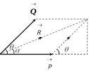 \[|\overrightarrow{R}|=R=\sqrt{{{P}^{2}}+{{Q}^{2}}+2PQ\,\cos \theta }\]
where \[|\overrightarrow{P}|=P,\,|\overrightarrow{Q}|=Q,\]
Also, \[\tan \alpha =\frac{Q\sin \theta }{P+Q\cos \theta }\]
Deduction : When \[|\overrightarrow{P}|=|\overrightarrow{Q}|\], more...
\[|\overrightarrow{R}|=R=\sqrt{{{P}^{2}}+{{Q}^{2}}+2PQ\,\cos \theta }\]
where \[|\overrightarrow{P}|=P,\,|\overrightarrow{Q}|=Q,\]
Also, \[\tan \alpha =\frac{Q\sin \theta }{P+Q\cos \theta }\]
Deduction : When \[|\overrightarrow{P}|=|\overrightarrow{Q}|\], more...  Magnitude or modulus of \[\mathbf{a}\] is expressed as
\[|\mathbf{a}|=|\overrightarrow{AB}|=AB\].
Magnitude or modulus of \[\mathbf{a}\] is expressed as
\[|\mathbf{a}|=|\overrightarrow{AB}|=AB\]. 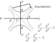 (iv) The equation of the pair of asymptotes differ the hyperbola and the conjugate hyperbola by the same constant only i.e., Hyperbola – Asymptotes = Asymptotes – Conjugated hyperbola or
\[\left( \frac{{{x}^{2}}}{{{a}^{2}}}-\frac{{{y}^{2}}}{{{b}^{2}}}-1 \right)-\left( \frac{{{x}^{2}}}{{{a}^{2}}}-\frac{{{y}^{2}}}{{{b}^{2}}} \right)=\left( \frac{{{x}^{2}}}{{{a}^{2}}}-\frac{{{y}^{2}}}{{{b}^{2}}} \right)-\left( \frac{{{x}^{2}}}{{{a}^{2}}}-\frac{{{y}^{2}}}{{{b}^{2}}}+1 \right)\].
(v) The asymptotes pass through the centre of the hyperbola.
(vi) The bisectors of the angles between the asymptotes are the coordinate axes.
(vii) The angle between the asymptotes of the hyperbola \[S=0\] i.e., \[\frac{{{x}^{2}}}{{{a}^{2}}}-\frac{{{y}^{2}}}{{{b}^{2}}}=1\] is \[2{{\tan }^{-1}}\frac{b}{a}\] or 2\[{{\sec }^{-1}}e\].
(viii) Asymptotes are equally inclined to the axes of the hyperbola.
(iv) The equation of the pair of asymptotes differ the hyperbola and the conjugate hyperbola by the same constant only i.e., Hyperbola – Asymptotes = Asymptotes – Conjugated hyperbola or
\[\left( \frac{{{x}^{2}}}{{{a}^{2}}}-\frac{{{y}^{2}}}{{{b}^{2}}}-1 \right)-\left( \frac{{{x}^{2}}}{{{a}^{2}}}-\frac{{{y}^{2}}}{{{b}^{2}}} \right)=\left( \frac{{{x}^{2}}}{{{a}^{2}}}-\frac{{{y}^{2}}}{{{b}^{2}}} \right)-\left( \frac{{{x}^{2}}}{{{a}^{2}}}-\frac{{{y}^{2}}}{{{b}^{2}}}+1 \right)\].
(v) The asymptotes pass through the centre of the hyperbola.
(vi) The bisectors of the angles between the asymptotes are the coordinate axes.
(vii) The angle between the asymptotes of the hyperbola \[S=0\] i.e., \[\frac{{{x}^{2}}}{{{a}^{2}}}-\frac{{{y}^{2}}}{{{b}^{2}}}=1\] is \[2{{\tan }^{-1}}\frac{b}{a}\] or 2\[{{\sec }^{-1}}e\].
(viii) Asymptotes are equally inclined to the axes of the hyperbola. 


You need to login to perform this action.
You will be redirected in
3 sec

