Current Affairs JEE Main & Advanced

In a quadratic equation \[a{{x}^{2}}+bx+c=0\], let us suppose that \[a,b,c\] are real and \[a\ne 0\]. The following is true about the nature of its roots.   (1) The equation has real and distinct roots if and only if \[D\equiv {{b}^{2}}-4ac>0\].   (2) The equation has real and coincident (equal) roots if and only if \[D\equiv {{b}^{2}}-4ac=0\].   (3) The equation has complex roots of the form \[\alpha \pm i\beta ,\,\alpha \ne 0,\] \[\beta \ne 0\in R\]  if and only if \[D\equiv {{b}^{2}}-4ac<0.\]   (4) The equation has rational roots if and only if \[a,b,c\in Q\] (the set of rational numbers) and \[D\equiv {{b}^{2}}-4ac\] is a perfect square (of a rational number).   (5) The equation has (unequal) irrational (surd form) roots if and only if \[D\equiv {{b}^{2}}-4ac>0\] and not a perfect square even if a, b and c are rational. In this case if \[p+\sqrt{q}\], \[p,q\] rational is an irrational root, then \[p-\sqrt{q}\] is also a root (a, b, c being rational).   (6) \[\alpha +i\beta \] (\[\beta \ne 0\] and \[\alpha ,\beta \in R\]) is a root if and only if its conjugate \[\alpha -i\beta \] is a root, that is complex roots occur in pairs in a quadratic equation. In case the equation is satisfied by more than two complex numbers, then it reduces to an identity. \[0.{{x}^{2}}+0.x+0=0\], i.e., \[a=0=b=c\].

(1) Relation between roots and coefficients of quadratic equation : If \[\alpha \] and \[\beta \] are the roots of quadratic equation \[a{{x}^{2}}+bx+c=0\], \[(a\ne 0)\] then   Sum of roots \[=S=\alpha +\beta =\frac{-b}{a}=-\frac{\text{Coefficien}\text{t of }x}{\text{Coefficien}\text{t of }{{x}^{2}}}\]   Product of roots \[=P=\alpha .\beta =\frac{c}{a}=\frac{\text{Constant term}}{\text{Coefficient of }{{x}^{2}}}\]   (2) Formation of an equation with given roots : A quadratic equation whose roots are \[\alpha \] and \[\beta \] is given by \[(x-\alpha )(x-\beta )=0\].   \[\therefore \] \[{{x}^{2}}-(\alpha +\beta )x+\alpha \beta =0\]   i.e. \[{{x}^{2}}-(\text{sum of roots)}x+(\text{product of roots})=0\]   \[\therefore \] \[{{x}^{2}}-Sx+P=0\]   (3) Symmetric function of the roots : A function of \[\alpha \] and \[\beta \] is said to be a symmetric function, if it remains unchanged when \[\alpha \] and \[\beta \] are interchanged.   For example, \[{{\alpha }^{2}}+{{\beta }^{2}}+2\alpha \beta \] is a symmetric function of \[\alpha \] and \[\beta \] whereas \[{{\alpha }^{2}}-{{\beta }^{2}}+3\alpha \beta \] is not a symmetric function of  \[\alpha \] and \[\beta \].   In order to find the value of a symmetric function of \[\alpha \] and \[\beta \], express the given function in terms of \[\alpha +\beta \] and \[\alpha \beta \]. The following results may be useful.   (i)   \[a\]   (ii) \[{{\alpha }^{3}}+{{\beta }^{3}}={{(\alpha +\beta )}^{3}}-3\alpha \beta (\alpha +\beta )\]   (iii) \[{{\alpha }^{4}}+{{\beta }^{4}}=({{\alpha }^{3}}+{{\beta }^{3}})(\alpha +\beta )-\alpha \beta ({{\alpha }^{2}}+{{\beta }^{2}})\]   (iv) \[{{\alpha }^{5}}+{{\beta }^{5}}=({{\alpha }^{3}}+{{\beta }^{3}})({{\alpha }^{2}}+{{\beta }^{2}})-{{\alpha }^{2}}{{\beta }^{2}}(\alpha +\beta )\]   (v)  \[|\alpha -\beta |=\sqrt{{{(\alpha +\beta )}^{2}}-4\alpha \beta }\]   (vi) \[{{\alpha }^{2}}-{{\beta }^{2}}=(\alpha +\beta )(\alpha -\beta )\]   (vii)  \[{{\alpha }^{3}}-{{\beta }^{3}}=(\alpha -\beta )[{{(\alpha +\beta )}^{2}}-\alpha \beta ]\]   (viii) \[{{\alpha }^{4}}-{{\beta }^{4}}=(\alpha +\beta )(\alpha -\beta )({{\alpha }^{2}}+{{\beta }^{2}})\]

The equation \[p(x)={{a}_{0}}{{x}^{n}}+{{a}_{1}}{{x}^{n-1}}+.....+{{a}_{n-1}}x+{{a}_{n}}=0\]…..(i)   Where the coefficients \[{{a}_{0}},{{a}_{1}},.......,{{a}_{n}}\in R\] (or C) and \[{{a}_{0}}\ne 0\] is called an equation of \[{{n}^{th}}\] degree, which has exactly \[n\] roots \[{{\alpha }_{1}},\,{{\alpha }_{2}},........,{{\alpha }_{n}}\in C\], then we can write \[p(x)={{a}_{0}}(x-{{\alpha }_{1}})\,(x-{{\alpha }_{2}})......(x-{{\alpha }_{n}})\]   = \[{{a}_{0}}\{{{x}^{n}}-(\Sigma {{\alpha }_{1}}){{x}^{n-1}}+(\Sigma {{\alpha }_{1}}{{\alpha }_{2}}){{x}^{n-2}}-.....+{{(-1)}^{n}}{{\alpha }_{1}}{{\alpha }_{2}}.....{{\alpha }_{n}}\}\]                                                                                       …(ii)   Comparing (i) and (ii), \[\Sigma {{\alpha }_{1}}={{\alpha }_{1}}+{{\alpha }_{2}}+.......+{{\alpha }_{n}}=-\frac{{{a}_{1}}}{{{a}_{0}}}\]   \[\Sigma {{\alpha }_{1}}{{\alpha }_{2}}={{\alpha }_{1}}{{\alpha }_{2}}+.....+{{\alpha }_{n-1}}{{\alpha }_{n}}=\frac{{{a}_{2}}}{{{a}_{0}}}\]   and so on and \[{{\alpha }_{1}}{{\alpha }_{2}}.....{{\alpha }_{n}}={{(-1)}^{n}}\frac{{{a}_{n}}}{{{a}_{0}}}\]   Cubic equation : When \[n=3\], the equation is a cubic of the form \[a{{x}^{3}}+b{{x}^{2}}+cx+d=0\], and we have in this case \[\alpha +\beta +\gamma =-\frac{b}{a};\] \[\alpha \beta +\beta \gamma +\gamma \alpha =\frac{c}{a};\,\text{  }\alpha \beta \gamma =-\frac{d}{a}\]   Biquadratic equation : If \[\alpha ,\beta ,\gamma ,\delta \] are roots of the biquadratic equation \[a{{x}^{4}}+b{{x}^{3}}+c{{x}^{2}}+dx+e=0\], then \[{{\sigma }_{1}}=\alpha +\beta +\gamma +\delta =-\frac{b}{a}\]   \[{{\sigma }_{2}}=\alpha \beta +\alpha \gamma +\alpha \delta +\beta \gamma +\beta \delta +\gamma \delta =\frac{c}{a}\]   \[{{\sigma }_{3}}=\alpha \beta \gamma +\alpha \beta \delta +\alpha \gamma \delta +\beta \gamma \delta =-\frac{d}{a}\]   \[{{\sigma }_{4}}=\alpha \beta \gamma \delta =\frac{e}{a}\].   Formation of a polynomial equation from given roots : If \[{{\alpha }_{1}},{{\alpha }_{2}},{{\alpha }_{3}},.....{{\alpha }_{n}}\]are the roots of a polynomial equation of degree n, then the equation is   \[{{x}^{n}}-{{\sigma }_{1}}{{x}^{n-1}}+{{\sigma }_{2}}{{x}^{n-2}}-{{\sigma }_{3}}{{x}^{n-3+......+}}{{(-1)}^{n}}{{\sigma }_{n}}=0\]   where \[{{\sigma }_{r}}=\sum{{{\alpha }_{1}}}{{\alpha }_{2}}.....{{\alpha }_{r}}.\]   Cubic equation : If \[\alpha ,\beta ,\gamma \] are the roots of a cubic equation, then the equation is \[{{x}^{3}}-{{\sigma }_{1}}{{x}^{2}}+{{\sigma }_{2}}x-{{\sigma }_{3}}=0\] or \[{{x}^{3}}-(\alpha +\beta +\gamma ){{x}^{2}}+(\alpha \beta +\alpha \gamma +\beta \gamma )x-\alpha \beta \gamma =0\].   Biquadratic Equation : If \[\alpha ,\beta ,\gamma ,\delta \] are the roots of a biquadratic equation, then the equation is   \[{{x}^{4}}-{{\sigma }_{1}}{{x}^{3}}+{{\sigma }_{2}}{{x}^{2}}-{{\sigma }_{3}}x+{{\sigma }_{4}}=0\]   or  \[{{x}^{4}}-(\alpha +\beta +\gamma +\delta ){{x}^{3}}+(\alpha \beta +\alpha \gamma +\alpha \delta \]   \[+\beta \gamma +\beta \delta +\gamma \delta ){{x}^{2}}-(\alpha \beta \gamma +\alpha \beta \delta +\alpha \gamma \delta +\beta \gamma \delta )\]\[x+\alpha \beta \gamma \delta =0\]

(1) Only one root is common : Let \[\alpha \] be the common root of quadratic equations \[{{a}_{1}}{{x}^{2}}+{{b}_{1}}x+{{c}_{1}}=0\] and \[{{a}_{2}}{{x}^{2}}+{{b}_{2}}x+{{c}_{2}}=0\].   \[\therefore \] \[{{a}_{1}}{{\alpha }^{2}}+{{b}_{1}}\alpha +{{c}_{1}}=0\], \[{{a}_{2}}{{\alpha }^{2}}+{{b}_{2}}\alpha +{{c}_{2}}=0\]   By Crammer’s rule : \[\frac{{{\alpha }^{2}}}{\left| \,\begin{matrix} -{{c}_{1}} & {{b}_{1}}  \\ -{{c}_{2}} & {{b}_{2}}  \\ \end{matrix}\, \right|}=\frac{\alpha }{\left| \,\begin{matrix} {{a}_{1}} & -{{c}_{1}}  \\ {{a}_{2}} & -{{c}_{2}}  \\ \end{matrix}\, \right|}=\frac{1}{\left| \,\begin{matrix} {{a}_{1}} & {{b}_{1}}  \\ {{a}_{2}} & {{b}_{2}}  \\ \end{matrix}\, \right|}\]   or \[\frac{{{\alpha }^{2}}}{{{b}_{1}}{{c}_{2}}-{{b}_{2}}{{c}_{1}}}=\frac{\alpha }{{{a}_{2}}{{c}_{1}}-{{a}_{1}}{{c}_{2}}}=\frac{1}{{{a}_{1}}{{b}_{2}}-{{a}_{2}}{{b}_{1}}}\]   \[\therefore \] \[\alpha =\frac{{{a}_{2}}{{c}_{1}}-{{a}_{1}}{{c}_{2}}}{{{a}_{1}}{{b}_{2}}-{{a}_{2}}{{b}_{1}}}=\frac{{{b}_{1}}{{c}_{2}}-{{b}_{2}}{{c}_{1}}}{{{a}_{2}}{{c}_{1}}-{{a}_{1}}{{c}_{2}}}\], \[\alpha \ne 0\]   \[\therefore \] The condition for only one root common is   \[{{({{c}_{1}}{{a}_{2}}-{{c}_{2}}{{a}_{1}})}^{2}}=({{b}_{1}}{{c}_{2}}-{{b}_{2}}{{c}_{1}})({{a}_{1}}{{b}_{2}}-{{a}_{2}}{{b}_{1}})\]   (2) Both roots are common: Then required condition is   \[\frac{{{a}_{1}}}{{{a}_{2}}}=\frac{{{b}_{1}}}{{{b}_{2}}}=\frac{{{c}_{1}}}{{{c}_{2}}}\]

(1) If \[f(a)\] and \[f(b)\] are of opposite signs then at least one or in general odd number of roots of the equation \[f(x)=0\] lie between \[a\] and \[b\].   (2) If \[f(a)=f(b)\] then there exists a point \[c\] between \[a\] and \[b\] such that \[{f}'(c)=0\], \[a<c<b\].   (3) If \[\alpha \] is a root of the equation \[f(x)=0\] then the polynomial \[f(x)\] is exactly divisible by \[(x-\alpha )\], then \[(x-\alpha )\] is factor of \[f(x)\].   (4) If the roots of the quadratic equations \[{{a}_{1}}{{x}^{2}}+{{b}_{1}}x+{{c}_{1}}=0\] and \[{{a}_{2}}{{x}^{2}}+{{b}_{2}}x+{{c}_{2}}=0\] are in the same ratio \[\left( i.e.\,\,\frac{{{\alpha }_{1}}}{{{\beta }_{1}}}=\frac{{{\alpha }_{2}}}{{{\beta }_{2}}} \right)\]  then \[b_{1}^{2}/b_{2}^{2}={{a}_{1}}{{c}_{1}}/{{a}_{2}}{{c}_{2}}\].

(1) Let \[f(x)\equiv a{{x}^{2}}+bx+c,\] \[a,b,c\in R\], \[a>0\] be a quadratic expression. Since, \[f(x)=a\,\left\{ {{\left( x+\frac{b}{2a} \right)}^{2}}-\left( \frac{{{b}^{2}}-4ac}{4{{a}^{2}}} \right) \right\}\] ……(i) The following is true from equation (i)   (i) \[f(x)>0\,\,(<0)\] for all values of \[x\in R\] if and only if   \[a>0\,(<0)\]  and \[D\equiv {{b}^{2}}-4ac<0\].   (ii) \[f(x)\ge 0\,(\le 0)\] if and only if   \[a>0\,(<0)\] and \[D\equiv {{b}^{2}}-4ac=0\].   In this case \[(D=0)\], \[f(x)=0\] if and only if \[x=-\frac{b}{2a}\]   (iii) If \[D\equiv {{b}^{2}}-4ac>0\] and \[a>0\,\,(<0),\] then   \[f(x)\,\left[ \begin{matrix} <0(>0), & \text{for }x\,\text{lying betw}\text{een the roots of }f(x)=0\,\,\,\,\,\,\,\,  \\ >0(<0), & \text{for }x\,\text{not lying betw}\text{een the roots of }f(x)=0  \\ =0, & \text{for }x=\text{each of the roots of }f(x)=0\,\,\,\,\,\,\,\,\,\,\,\,\,\,\,\,\,\,  \\ \end{matrix} \right.\]   (iv) If \[a>0,\,(<0)\], then \[f(x)\] has a minimum (maximum) value at \[x=-\frac{b}{2a}\] and this value is given by   \[{{[f(x)]}_{\text{min}\,\text{(max)}}}=\frac{4ac-{{b}^{2}}}{4a}\].   (2) Sign of quadratic expression : Let \[f(x)=a{{x}^{2}}+bx+c\] or \[y=a{{x}^{2}}+bx+c\]   Where \[a,\,b,\,\,c\,\,\in R\] and \[a\ne 0,\] for some values of \[x,\,\,f(x)\] may be positive, negative or zero. 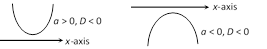This gives the following cases :   (i) \[a>0\] and \[D<0,\] so \[f(x)>0\] for all \[x\in R\] i.e., \[f(x)\] is positive for all real values of \[x\].     (ii) \[a<0\] and \[D<0,\] so \[f(x)<0\] for all \[x\in R\] i.e., \[f(x)\] is negative for all real values of \[x\].   (iii) \[a>0\] and \[D=0,\] so \[f(x)\ge 0\] for all \[x\in R\] i.e., \[f(x)\] is positive for all real values of \[x\] except at vertex, where \[f(x)=0\].   (iv) \[a<0\]  and \[D=0,\] so \[f(x)\le 0\] for all \[x\in R\] i.e. \[f(x)\] is negative for all real values of \[x\] except at vertex, where \[f(x)=0\].   (v) \[a>0\] and \[D>0,\] let \[f(x)=0\] have two real roots \[\alpha \] and \[\beta \] \[(\alpha <\beta ),\] then \[f(x)>0\] for all \[x\in (-\infty ,\,\alpha )\cup (\beta ,\,\infty )\] and \[f(x)<0\] for all \[x\in (\alpha ,\,\beta )\]. (vi) \[a<0\] and \[D>0\], let \[f(x)=0\] have two real roots \[\alpha \] and \[\beta \]\[(\alpha <\beta )\]. Then x\[f(x)<0\] for all \[x\in (-\infty ,\,\alpha )\cup (\beta ,\,\infty )\] and \[f(x)>0\] for all \[x\in (\alpha ,\,\beta )\]   (3) Graph of a quadratic expression   We have \[y=a{{x}^{2}}+bx+c=f(x)\] . \[y=a\left[ {{\left( x+\frac{b}{2a} \right)}^{2}}-\frac{D}{4{{a}^{2}}} \right]\]\[\Rightarrow \] \[y+\frac{D}{4a}=a{{\left( x+\frac{b}{2a} \right)}^{2}}\]   Now, let \[y+\frac{D}{4a}=Y\] and \[X=x+\frac{b}{2a}\]   \[Y=a.{{X}^{2}}\]\[\Rightarrow \] \[{{X}^{2}}=\frac{1}{a}Y\]   (i) The graph of the curve \[y=f(x)\] is parabolic.   (ii) The axis of parabola is \[X=0\] or \[x+\frac{b}{2a}=0\]   i.e. (parallel to y-axis).   (iii) (a) If \[a>0,\] then the parabola opens upward.   (b) If \[a<0,\] then the parabola opens downward.                 (iv) Intersection with axis   (a) Intersection with x-axis : For \[x\] axis, \[y=0\]   \[\Rightarrow \] \[a{{x}^{2}}+bx+c=0\]\[\Rightarrow \]\[x=\frac{-b\pm \sqrt{D}}{2a}\]   For \[D>0,\] parabola cuts x-axis in two real and distinct points i.e.\[x=\frac{-b\pm \sqrt{D}}{2a}\].   For \[D=0,\] parabola touches x-axis in one point, \[x=-b/2a\].           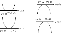For \[D<0,\] parabola does not cut x-axis (i.e. imaginary value of more...

Let \[f(x)={{(x-{{a}_{1}})}^{{{k}_{1}}}}{{(x-{{a}_{2}})}^{{{k}_{2}}}}{{(x-{{a}_{3}})}^{{{k}_{3}}}}......\]\[{{(x-{{a}_{n-1}})}^{{{k}_{n-1}}}}{{(x-{{a}_{n}})}^{{{k}_{n}}}}\]                                         …..(i)   where \[{{k}_{1}},\,{{k}_{2}},\,{{k}_{3}}...,\,{{k}_{n}}\in N\] and \[{{a}_{1}},\,{{a}_{2}},\,{{a}_{3}},\,......,\,{{a}_{n}}\] are fixed natural numbers satisfying the condition \[{{a}_{1}}<{{a}_{2}}<{{a}_{3}}.....<{{a}_{n-1}}<{{a}_{n}}\]   First we mark the numbers \[{{a}_{1}},\,{{a}_{2}},\,{{a}_{3}},\,......,\,{{a}_{n}}\] on the real axis and the plus sign in the interval of the right of the largest of these numbers, i.e. on the right of \[{{a}_{n}}\]. If \[{{k}_{n}}\] is even then we put plus sign on the left of \[{{a}_{n}}\] and if \[{{k}_{n}}\] is odd then we put minus sign on the left of \[{{a}_{n}}\]. In the next interval we put a sign according to the following rule :   When passing through the point \[{{a}_{n-1}}\] the polynomial \[f(x)\] changes sign if \[{{k}_{n-1}}\] is an odd number and the polynomial \[f(x)\] has same sign if \[{{k}_{n-1}}\] is an even number. Then, we consider the next interval and put a sign in it using the same rule. Thus, we consider all the intervals. The solution of \[f(x)>0\] is the union of all intervals in which we have put the plus sign and the solution of \[f(x)<0\] is the union of all intervals in which we have put the minus sign.

(1) If \[f(x)=0\] is an equation and \[a,b\] are two real numbers such that \[f(a).f(b)<0\] has at least one real root or an odd number of real roots between \[a\] and \[b\]. In case \[f(a)\] and \[f(b)\] are of the same sign, then either no real root or an even number of real roots of \[f(x)=0\]lie between a and b.     (2) Every equation of an odd degree has at least one real root, whose sign is opposite to that of its last term, provided the coefficient of the first term is \[+ve\] e.g., \[{{x}^{3}}-3x+2=0\] has one real negative root.     (3) Every equation of an even degree whose last term is \[-ve\]  and the coefficient of first term \[+ve\] has at least two real roots, one \[+ve\] and one \[-ve\] e.g., \[{{x}^{4}}+4{{x}^{3}}+3{{x}^{2}}+5x-2=0\] has at least two real roots, one \[+ve\] and one \[-ve\].     (4) If an equation has only one change of sign, it has one \[+ve\] root and no more.     (5) If all the terms of an equation are \[+ve\] and the equation involves no odd power of \[x,\] then all its roots are complex.

The maximum number of positive real roots of a polynomial equation \[f(x)=0\] is the number of changes of sign from positive to negative and negative to positive in \[f(x)\].   The maximum number of negative real roots of a polynomial equation \[f(x)=0\] is the number of changes of sign from positive to negative and negative to positive in \[f(-x)\].

(1) Values of rational expression \[P(x)/Q(x)\] for real values of \[x,\] where \[P(x)\] and \[Q(x)\] are quadratic expressions : To find the values attained by rational expression of the form \[\frac{{{a}_{1}}{{x}^{2}}+{{b}_{1}}x+{{c}_{1}}}{{{a}_{2}}{{x}^{2}}+{{b}_{2}}x+{{c}_{2}}}\] for real values of \[x,\] the following algorithm will explain the procedure :   Algorithm   Step I: Equate the given rational expression to \[y\].   Step II: Obtain a quadratic equation in \[x\] by simplifying the expression in step I.   Step III: Obtain the discriminant of the quadratic equation in Step II.   Step IV: Put Discriminant \[\ge 0\] and solve the inequation for \[y\]. The values of \[y\] so obtained determines the set of values attained by the given rational expression.   (2) Solution of rational algebraic inequation: If \[P(x)\] and \[Q(x)\] are polynomial in \[x,\] then the inequation   \[\frac{P(x)}{Q(x)}>0,\,\frac{P(x)}{Q(x)}<0,\,\frac{P(x)}{Q(x)}\ge 0\] and \[\frac{P(x)}{Q(x)}\le 0\]   are known as rational algebraic inequations.   To solve these inequations we use the sign method as explained in the following algorithm.   Algorithm   Step I: Obtain \[P(x)\] and \[Q(x)\].   Step II: Factorize \[P(x)\] and \[Q(x)\] into linear factors.   Step III: Make the coefficient of \[x\] positive in all factors.   Step IV: Obtain critical points by equating all factors to zero.   Step V: Plot the critical points on the number line. If there are \[n\] critical points, they divide the number line into \[(n+1)\] regions.   Step VI: In the right most region the expression \[\frac{P(x)}{Q(x)}\] bears positive sign and in other regions the expression bears positive and negative signs depending on the exponents of the factors.   (3) Lagrange’s identity   If \[{{a}_{1}},\,{{a}_{2}},\,{{a}_{3}},\,{{b}_{1}},\,{{b}_{2}},\,{{b}_{3}}\in R\] then    \[(a_{1}^{2}+a_{2}^{2}+a_{3}^{2})(b_{1}^{2}+b_{2}^{2}+b_{3}^{2})-{{({{a}_{1}}{{b}_{1}}+{{a}_{2}}{{b}_{2}}+{{a}_{3}}{{b}_{3}})}^{2}}\]   \[={{({{a}_{1}}{{b}_{2}}-{{a}_{2}}{{b}_{1}})}^{2}}+{{({{a}_{2}}{{b}_{3}}-{{a}_{3}}{{b}_{2}})}^{2}}+{{({{a}_{3}}{{b}_{1}}-{{a}_{1}}{{b}_{3}})}^{2}}\]