| Trigonometrical equation | General solution |
| \[\sin \theta =0\] | \[\theta =n\pi \] |
| \[\cos \theta =0\] | \[\theta =n\pi +\pi /2\] |
| \[\tan \theta =0\] | \[\theta =n\pi \] |
| \[\sin \theta =1\] | \[\theta =2n\pi +\pi /2\] |
| \[\cos \theta =1\] | \[\theta =2n\pi \] |
| \[\sin \theta =\sin \alpha \] | \[\theta =n\pi +{{(-1)}^{n}}\alpha \] |
| \[\cos \theta =\cos \alpha \] | \[\theta =2n\pi \pm \alpha \] |
| \[\tan \theta =\tan \alpha \] | \[\theta =n\pi \pm \alpha \] |
| \[{{\sin }^{2}}\theta ={{\sin }^{2}}\alpha \] | \[\theta =n\pi \pm \alpha \] |
| \[{{\tan }^{2}}\theta ={{\tan }^{2}}\alpha \] | \[\theta =n\pi \pm \alpha \] |
| \[{{\cos }^{2}}\theta ={{\cos }^{2}}\alpha \] | \[\theta =n\pi \pm \alpha \] |
| \[\left. \begin{align} & \sin \theta =\sin \alpha \\ & \cos \theta =\cos \alpha \text{ } \\ \end{align} \right|\text{ * }\] | more...
An equation involving one or more trigonometrical ratio of an unknown angle is called a trigonometrical equation
i.e., \[\sin x+\cos 2x=1\],\[(1-\tan \theta )(1+\sin 2\theta )=1+\tan \theta \], \[|\sec \left( \theta +\frac{\pi }{4} \right)|\text{ }=2\] etc.
A trigonometric equation is different from a trigonometrical identities. An identity is satisfied for every value of the unknown angle e.g.,\[{{\cos }^{2}}x=1-{{\sin }^{2}}x\]is true \[\forall x\in R\], while a trigonometric equation is satisfied for some particular values of the unknown angle.
(1) Roots of trigonometrical equation : The value of unknown angle (a variable quantity) which satisfies the given equation is called the root of an equation, e.g., \[\cos \theta =\frac{1}{2}\], the root is \[\theta ={{60}^{o}}\] or \[\theta ={{300}^{o}}\] because the equation is satisfied if we put \[\theta ={{60}^{o}}\]or \[\theta ={{300}^{o}}\].
(2) Solution of trigonometrical equations : A value of the unknown angle which satisfies the trigonometrical equation is called its solution.
Since all trigonometrical ratios are periodic in nature, generally a trigonometrical equation has more than one solution or an infinite number of solutions. There are basically three types of solutions:
(i) Particular solution : A specific value of unknown angle satisfying the equation.
(ii) Principal solution : Smallest numerical value of the unknown angle satisfying the equation (Numerically smallest particular solution).
(iii) General solution : Complete set of values of the unknown angle satisfying the equation. It contains all particular solutions as well as principal solutions.
The function, \[f(x)\] is differentiable at point \[P,\] iff there exists a unique tangent at point \[P\]. In other words, \[f(x)\] is differentiable at a point \[P\] iff the curve does not have \[P\] as a corner point. i.e., "the function is not differentiable at those points on which function has jumps (or holes) and sharp edges.”
Let us consider the function \[f(x)=|x-1|\], which can be graphically shown,
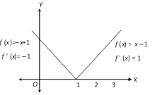 Which show \[f(x)\] is not differentiable at \[x=1\]. Since, \[f(x)\]has sharp edge at \[x=1\].
(i) Right hand derivative : Right hand derivative of \[f(x)\] at \[x=a\], denoted by \[f'(a+0)\] or \[f'(a+)\], is the \[\underset{h\to 0}{\mathop{\lim }}\,\frac{f(a+h)-f(a)}{h}\].
(ii) Left hand derivative : Left hand derivative of \[f(x)\] at \[x=a,\] denoted by \[f'(a-0)\] or \[f'(a-)\], is the \[\underset{h\to 0}{\mathop{\lim }}\,\,\frac{f(a-h)-f(a)}{-h}\].
(iii) A function \[f(x)\] is said to be differentiable (finitely) at \[x=a\] if \[f'(a+0)=f'(a-0)\]= finite
i.e., \[\underset{h\to 0}{\mathop{\lim }}\,\,\frac{f(a+h)-f(a)}{h}=\underset{h\to 0}{\mathop{\lim }}\,\frac{f(a-h)-f(a)}{-h}\] = finite and the common limit is called the derivative of \[f(x)\] at \[x=a\], denoted by \[f'(a)\]. Clearly, \[f'(a)=\underset{x\to a}{\mathop{\lim }}\,\frac{f(x)-f(a)}{x-a}\] {x \[\to \] a from the left as well as from the right}.
Some standard results on differentiability
(1) Every polynomial function is differentiable at each \[x\in R\].
(2) The exponential function \[{{a}^{x}},a>0\] is differentiable at each \[x\in R\].
(3) Every constant function is differentiable at each \[x\in R\].
(4) The logarithmic function is differentiable at each point in its domain.
(5) Trigonometric and inverse trigonometric functions are differentiable in their domains.
(6) The sum, difference, product and quotient of two differentiable functions is differentiable.
(7) The composition of differentiable function is a differentiable function.
Which show \[f(x)\] is not differentiable at \[x=1\]. Since, \[f(x)\]has sharp edge at \[x=1\].
(i) Right hand derivative : Right hand derivative of \[f(x)\] at \[x=a\], denoted by \[f'(a+0)\] or \[f'(a+)\], is the \[\underset{h\to 0}{\mathop{\lim }}\,\frac{f(a+h)-f(a)}{h}\].
(ii) Left hand derivative : Left hand derivative of \[f(x)\] at \[x=a,\] denoted by \[f'(a-0)\] or \[f'(a-)\], is the \[\underset{h\to 0}{\mathop{\lim }}\,\,\frac{f(a-h)-f(a)}{-h}\].
(iii) A function \[f(x)\] is said to be differentiable (finitely) at \[x=a\] if \[f'(a+0)=f'(a-0)\]= finite
i.e., \[\underset{h\to 0}{\mathop{\lim }}\,\,\frac{f(a+h)-f(a)}{h}=\underset{h\to 0}{\mathop{\lim }}\,\frac{f(a-h)-f(a)}{-h}\] = finite and the common limit is called the derivative of \[f(x)\] at \[x=a\], denoted by \[f'(a)\]. Clearly, \[f'(a)=\underset{x\to a}{\mathop{\lim }}\,\frac{f(x)-f(a)}{x-a}\] {x \[\to \] a from the left as well as from the right}.
Some standard results on differentiability
(1) Every polynomial function is differentiable at each \[x\in R\].
(2) The exponential function \[{{a}^{x}},a>0\] is differentiable at each \[x\in R\].
(3) Every constant function is differentiable at each \[x\in R\].
(4) The logarithmic function is differentiable at each point in its domain.
(5) Trigonometric and inverse trigonometric functions are differentiable in their domains.
(6) The sum, difference, product and quotient of two differentiable functions is differentiable.
(7) The composition of differentiable function is a differentiable function.
(1) Discontinuous function : A function \['f'\] which is not continuous at a point \[x=a\] in its domain is said to be discontinuous there at. The point \['a'\] is called a point of discontinuity of the function.
The discontinuity may arise due to any of the following situations.
(i) \[\underset{x\to {{a}^{+}}}{\mathop{\lim }}\,f(x)\] or \[\underset{x\to {{a}^{-}}}{\mathop{\lim }}\,f(x)\] or both may not exist
(ii) \[\underset{x\to {{a}^{+}}}{\mathop{\lim }}\,f(x)\]as well as \[\underset{x\to {{a}^{-}}}{\mathop{\lim }}\,f(x)\] may exist, but are unequal.
(iii)\[\underset{x\to {{a}^{+}}}{\mathop{\lim }}\,f(x)\] as well as \[\underset{x\to {{a}^{-}}}{\mathop{\lim }}\,f(x)\] both may exist, but either of the two or both may not be equal to \[f(a)\].
Function \[f(x)\] is said to be
(1) Left continuous at \[x=a\] if \[\underset{x\to {{a}^{-}}}{\mathop{\text{lim}}}\,f(x)=f(a)\]
(2) Right continuous at \[x=a\] if \[\underset{x\to {{a}^{+}}}{\mathop{\text{lim}}}\,f(x)=f(a)\].
Thus a function \[f(x)\] is continuous at a point \[x=a\] if it is left continuous as well as right continuous at \[x=a.\]
Properties of continuous functions : Let \[f(x)\] and \[g(x)\] be two continuous functions at \[x=a.\]Then
(i) A function \[f(x)\] is said to be everywhere continuous if it is continuous on the entire real line R i.e. \[(-\infty ,\infty )\]. e.g., polynomial function, \[{{e}^{x}},\]\[\sin x,\,\cos x,\,\]constant, \[{{x}^{n}},\] \[|x-a|\] etc.
(ii) Integral function of a continuous function is a continuous function.
(iii) If \[g(x)\] is continuous at \[x=a\] and \[f(x)\] is continuous at \[x=g(a)\] then \[(fog)\,(x)\] is continuous at \[x=a\].
(iv) If \[f(x)\] is continuous in a closed interval \[[a,\,\,b]\] then it is bounded on this interval.
(v) If \[f(x)\] is a continuous function defined on \[[a,\,\,b]\] such that \[f(a)\] and \[f(b)\] are of opposite signs, then there is atleast one value of \[x\] for which \[f(x)\] vanishes. i.e. if \[f(a)>0,\,\,f(b)<0\Rightarrow \,\exists \,\,c\,\,\in \,\,(a,\,\,b)\] such that \[f(c)\,=0\].
A function \[f(x)\] is said to be continuous at a point \[x=a\] of its domain if and only if it satisfies the following three conditions :
(1) \[f(a)\] exists. (\['a'\] lies in the domain of \[f\])
(2) \[\underset{x\to a}{\mathop{\lim }}\,\,f(x)\] exist i.e.\[\underset{x\to {{a}^{+}}}{\mathop{\lim }}\,f(x)=\underset{x\to {{a}^{-}}}{\mathop{\lim }}\,f(x)\] or R.H.L. = L.H.L.
(3) \[\underset{x\to a}{\mathop{\lim }}\,f(x)=f(a)\] (limit equals the value of function).
Cauchy’s definition of continuity : A function \[f\] is said to be continuous at a point \[a\] of its domain \[D\] if for every \[\varepsilon >0\] there exists \[\delta >0\] (dependent on \[\varepsilon )\] such that \[|x-a|<\delta \] \[\Rightarrow |\,f(x)-f(a)|<\varepsilon .\]
Comparing this definition with the definition of limit we find that \[f(x)\] is continuous at \[x=a\] if \[\underset{x\to a}{\mathop{\lim }}\,f(x)\] exists and is equal to \[f(a)\] i.e., if \[\underset{x\to {{a}^{-}}}{\mathop{\lim }}\,f(x)=f(a)=\underset{x\to a+}{\mathop{\lim }}\,f(x)\].
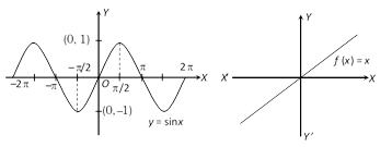
The word ‘continuous’ means without any break or gap. If the graph of a function has no break or gap or jump, then it is said to be continuous.
A function which is not continuous is called a discontinuous function. While studying graphs of functions, we see that graphs of functions \[\sin x\], \[x,\] \[\cos x\], \[{{e}^{x}}\] etc. are continuous but greatest integer function \[[x]\] has break at every integral point, so it is not continuous. Similarly \[\tan x,\,\,\cot x,\,\,\sec x\], \[\frac{1}{x}\] etc. are also discontinuous function.
Continuous function
 Discontinuous function
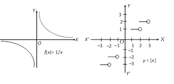
We shall divide the problems of evaluation of limits in five categories.
(1) Algebraic limits : Let \[f(x)\] be an algebraic function and \['a'\] be a real number. Then \[\underset{x\to a}{\mathop{\lim }}\,f(x)\] is known as an algebraic limit.
(i) Direct substitution method : If by direct substitution of the point in the given expression we get a finite number, then the number obtained is the limit of the given expression.
(ii) Factorisation method : In this method, numerator and denominator are factorised. The common factors are cancelled and the rest outputs the results.
(iii) Rationalisation method : Rationalisation is followed when we have fractional powers (like \[\frac{1}{2},\frac{1}{3}\] etc.) on expressions in numerator or denominator or in both. After rationalisation the terms are factorised which on cancellation gives the result.
(iv) Based on the form when \[x\to \infty \] : In this case expression should be expressed as a function \[1/x\] and then after removing indeterminate form, (if it is there) replace \[\frac{1}{x}\] by 0.
(2) Trigonometric limits : To evaluate trigonometric limit the following results are very important.
(i) \[\underset{x\to 0}{\mathop{\lim }}\,\,\frac{\sin x}{x}=1=\underset{x\to 0}{\mathop{\lim }}\,\,\frac{x}{\sin x}\]
(ii) \[\underset{x\to 0}{\mathop{\lim }}\,\,\frac{\tan x}{x}=1=\underset{x\to 0}{\mathop{\lim }}\,\,\frac{x}{\tan x}\]
(iii) \[\underset{x\to 0}{\mathop{\lim }}\,\,\frac{{{\sin }^{-1}}x}{x}=1=\underset{x\to 0}{\mathop{\lim }}\,\frac{x}{{{\sin }^{-1}}x}\]
(iv) \[\underset{x\to 0}{\mathop{\lim }}\,\frac{{{\tan }^{-1}}x}{x}=1=\underset{x\to 0}{\mathop{\lim }}\,\frac{x}{{{\tan }^{-1}}x}\]
(v) \[\underset{x\to 0}{\mathop{\lim }}\,\,\frac{\sin {{x}^{0}}}{x}=\frac{\pi }{180}\]
(vi) \[\underset{x\to 0}{\mathop{\lim }}\,\,\cos x=1\]
(vii) \[\underset{x\to a}{\mathop{\lim }}\,\,\frac{\sin (x-a)}{x-a}=1\]
(viii) \[\underset{x\to a}{\mathop{\lim }}\,\,\frac{\tan (x-a)}{x-a}=1\]
(ix) \[\underset{x\to a}{\mathop{\lim }}\,{{\sin }^{-1}}x={{\sin }^{-1}}a,\,\,|a|\,\,\le 1\]
(x) \[\underset{x\to a}{\mathop{\lim }}\,\,{{\cos }^{-1}}\,x={{\cos }^{-1}}\,a;\,\,|a|\,\,\le 1\]
(xi) \[\underset{x\to a}{\mathop{\lim }}\,\,{{\tan }^{-1}}\,x={{\tan }^{-1}}a;\,\,-\infty <a<\infty \]
(xii) \[\underset{x\to \infty }{\mathop{\lim }}\,\frac{\sin x}{x}=\underset{x\to \infty }{\mathop{\lim }}\,\frac{\cos x}{x}=0\]
(xiii) \[\underset{x\to \infty }{\mathop{\lim }}\,\frac{\sin \left( 1/x \right)}{\left( 1/x \right)}=1\]
(3) Logarithmic limits : To evaluate the logarithmic limits we use following formulae
(i) \[\log (1+x)=x-\frac{{{x}^{2}}}{2}+\frac{{{x}^{3}}}{3}-............\text{to}\,\infty \] where \[-1<x\le 1\] and expansion is true only if base is e.
(ii) \[\underset{x\to 0}{\mathop{\lim }}\,\,\frac{\log (1+x)}{x}=1\]
(iii) \[\underset{x\to e}{\mathop{\lim }}\,\,{{\log }_{e}}x=1\]
(iv) \[\underset{x\to 0}{\mathop{\lim }}\,\,\frac{\log (1-x)}{x}=-1\]
(v) \[\underset{x\to 0}{\mathop{\lim }}\,\frac{{{\log }_{a}}(1+x)}{x}={{\log }_{a}}e,\,a>0,\ne 1\]
(4) Exponential limits
(i) Based on series expansion
We use \[{{e}^{x}}=1+x+\frac{{{x}^{2}}}{2\,!}+\frac{{{x}^{3}}}{3\,!}+.............\infty \]
To evaluate the exponential limits we use the following results
(a) \[\underset{x\to 0}{\mathop{\lim }}\,\frac{{{e}^{x}}-1}{x}=1\]
(b) \[\underset{x\to 0}{\mathop{\lim }}\,\,\frac{{{a}^{x}}-1}{x}={{\log }_{e}}a\]
(c) \[\underset{x\to 0}{\mathop{\lim }}\,\,\frac{{{e}^{\lambda x}}-1}{x}=\,\lambda \,\,(\lambda \ne 0)\]
(ii) Based on the form \[{{1}^{\infty }}\] : To evaluate the exponential form \[{{1}^{\infty }}\] we use the following results.
(a) If \[\underset{x\to a}{\mathop{\lim }}\,\,f(x)=\underset{x\to a}{\mathop{\lim }}\,\,g(x)=0\], then
\[\underset{x\to a}{\mathop{\lim }}\,\,{{\{1+f(x)\}}^{1/g(x)}}\,\,=\,{{e}^{\underset{x\to a}{\mathop{\lim }}\,\,\frac{f(x)}{g(x)}}}\] or when \[\underset{x\to a}{\mathop{\lim }}\,\,f(x)=1\] and \[\underset{x\to a}{\mathop{\lim }}\,g(x)=\infty \].
Then \[\underset{x\to a}{\mathop{\lim }}\,{{\{f(x)\}}^{g(x)}}=\underset{x\to a}{\mathop{\lim }}\,\,{{[1+f(x)-1]}^{g(x)}}\]\[={{e}^{\underset{x\to a}{\mathop{\lim }}\,(f(x)-1)g(x)}}\]
(b) \[\underset{x\to 0}{\mathop{\lim }}\,{{(1+x)}^{1/x}}=e\]
(c) \[\underset{x\to \infty }{\mathop{\lim }}\,{{\left( more...
The following theorems are very useful for evaluation of limits if \[\underset{x\to 0}{\mathop{\lim }}\,f(x)=l\] and \[\underset{x\to 0}{\mathop{\lim }}\,g(x)=m\] (\[l\] and \[m\] are real numbers) then
(1) \[\underset{x\to a}{\mathop{\lim }}\,(f(x)+g(x))=l+m\,\] (Sum rule)
(2) \[\underset{x\to a}{\mathop{\lim }}\,(f(x)-g(x))=l-m\] (Difference rule)
(3) \[\underset{x\to a}{\mathop{\lim }}\,(f(x).g(x))=l.m\] (Product rule)
(4) \[\underset{x\to a}{\mathop{\lim }}\,k\,\,f(x)=k.l\] (Constant multiple rule)
(5) \[\underset{x\to a}{\mathop{\lim }}\,\,\frac{f(x)}{g(x)}=\frac{l}{m},m\ne 0\] (Quotient rule)
(6) If \[\underset{x\to a}{\mathop{\lim }}\,f(x)=+\infty \] or \[-\infty \], then \[\underset{x\to a}{\mathop{\lim }}\,\,\frac{1}{f(x)}=0\]
(7) \[\underset{x\to a}{\mathop{\lim }}\,\log \{f(x)\}=\log \,\{\underset{x\to a}{\mathop{\lim }}\,f(x)\}\]
(8) If \[f(x)\le g(x)\] for all \[x,\] then \[\underset{x\to a}{\mathop{\lim }}\,f(x)\le \underset{x\to a}{\mathop{\lim }}\,g(x)\]
(9) \[\underset{x\to a}{\mathop{\lim }}\,{{[f(x)]}^{g(x)}}={{\{\underset{x\to a}{\mathop{\lim }}\,f(x)\}}^{\underset{x\to a}{\mathop{\lim }}\,g(x)}}\]
(10) If \[p\] and \[q\] are integers, then \[\underset{x\to a}{\mathop{\lim }}\,{{(f(x))}^{p/q}}={{l}^{p/q}},\] provided \[{{(l)}^{p/q}}\] is a real number.
(11) If \[\underset{x\to a}{\mathop{\lim }}\,f(g(x))=f(\underset{x\to a}{\mathop{\lim }}\,g(x))=f(m)\] provided \['f'\] is continuous at \[g(x)=m.\,\,e.g.\]\[\underset{x\to a}{\mathop{\lim }}\,\ln [f(x)]=\ln (l),\]only if \[l>0.\]
Let \[y=f(x)\] be a function of \[x\]. If at \[x=a,f(x)\] takes indeterminate form, then we consider the values of the function which are very near to \['a'\]. If these values tend to a definite unique number as \[x\] tends to \['a'\], then the unique number so obtained is called the limit of \[f(x)\] at \[x=a\] and we write it as \[\underset{x\to a}{\mathop{\lim }}\,f(x)\].
(1) Left hand and right hand limit : Consider the values of the functions at the points which are very near to \[a\] on the left of \[a\]. If these values tend to a definite unique number as \[x\] tends to \[a,\] then the unique number so obtained is called left-hand limit of \[f(x)\] at \[x=a\] and symbolically we write it as \[f(a-0)=\]\[\underset{x\to {{a}^{-}}}{\mathop{\lim }}\,\,f(x)=\]\[\,\underset{h\to 0}{\mathop{\lim }}\,\,f(a-h)\].
Similarly we can define right-hand limit of \[f(x)\] at \[x=a\] which is expressed as \[f(a+0)=\underset{x\to {{a}^{+}}}{\mathop{\lim }}\,f(x)\]\[=\underset{h\to 0}{\mathop{\lim }}\,f(a+h)\].
(2) Method for finding L.H.L. and R.H.L.
(i) For finding right hand limit (R.H.L.) of the function, we write \[x+h\] in place of \[x,\] while for left hand limit (L.H.L.) we write \[x-h\] in place of \[x\].
(ii) Then we replace \[x\] by \['a'\] in the function so obtained.
(iii) Lastly we find limit \[h\to 0\].
(3) Existence of limit : \[\underset{x\to a}{\mathop{\lim }}\,f(x)\,\,\]exists when,
(i) \[\underset{x\to {{a}^{-}}}{\mathop{\lim }}\,f(x)\] and \[\underset{x\to {{a}^{+}}}{\mathop{\lim }}\,f(x)\] exist i.e. L.H.L. and R.H.L. both exists.
(ii) \[\underset{x\to {{a}^{-}}}{\mathop{\lim }}\,f(x)=\underset{x\to {{a}^{+}}}{\mathop{\lim }}\,f(x)\] i.e. L.H.L. = R.H.L.
Current Affairs CategoriesArchive
Trending Current Affairs


You need to login to perform this action. |

