Atomic Number, Mass Number and Atomic Species
(1) Atomic number or Nuclear charge
(i) The number of protons present in the nucleus of the atom is called atomic number (Z).
(ii) It was determined by Moseley as,
where, \[\nu =X-\]rays frequency
Z= atomic number of the metal
\[a\And b\] are constant.
(iii) Atomic number = Number of positive charge on nucleus = Number of protons in nucleus = Number of electrons in nutral atom.
(iv) Two different elements can never have identical atomic number.
(2) Mass number
(i) The sum of proton and neutrons present in the nucleus is called mass number.
Mass number (A) = Number of protons + Number of neutrons or Atomic number (Z)
or Number of neutrons = A – Z .
(ii) Since mass of a proton or a neutron is not a whole number (on atomic weight scale), weight is not necessarily a whole number.
(iii) The atom of an element X having mass number (A) and atomic number (Z) may be represented by a symbol,
Note : q A part of an atom up to penultimate shell is a kernel or atomic core.
q Negative ion is formed by gaining electrons and positive ion by the loss of electrons.
q Number of lost or gained electrons in positive or negative ion =Number of protons \[\pm \]charge on ion.
(3) Different Types of Atomic Species
Atomic Models and Planck's Quantum Theory
Atomic spectrum - Hydrogen spectrum.
Atomic spectrum
(1) Spectrum is the impression produced on a photographic film when the radiation (s) of particular wavelength (s) is (are) analysed through a prism or diffraction grating. It is of two types, emission and absorption.
(2) Emission spectrum : A substance gets excited on heating at a very high temperature or by giving energy and radiations are emitted. These radiations when analysed with the help of spectroscope, spectral lines are obtained. A substance may be excited, by heating at a higher temperature, by passing electric current at a very low pressure in a discharge tube filled with gas and passing electric current into metallic filament. Emission spectra is of two types,
(i) Continuous spectrum : When sunlight is passed through a prism, it gets dispersed into continuous bands of different colours. If the light of an incandescent object resolved through prism or spectroscope, it also gives continuous spectrum of colours.
(ii) Line spectrum : If the radiations obtained by the excitation of a substance are analysed with help of a spectroscope a series of thin bright lines of specific colours are obtained. There is dark space in between two consecutive lines. This type of spectrum is called line spectrum or atomic spectrum..
(3) Absorption spectrum : When the white light of an incandescent substance is passed through any substance, this substance absorbs the radiations of certain wavelength from the white light. On analysing the transmitted light we obtain a spectrum in which dark lines of specific wavelengths are observed. These lines constitute the absorption spectrum. The wavelength of the dark lines correspond to the wavelength of light absorbed.
Hydrogen spectrum
(1) Hydrogen spectrum is an example of line emission spectrum or atomic emission spectrum.
(2) When an electric discharge is passed through hydrogen gas at low pressure, a bluish light is emitted.
(3) This light shows discontinuous line spectrum of several isolated sharp lines through prism.
(4) All these lines of H-spectrum have Lyman, Balmer, Paschen, Barckett, Pfund and Humphrey series. These spectral series were named by the name of scientist discovered them.
(5) To evaluate wavelength of various H-lines Ritz introduced the following expression,
\[\bar{\nu }=\frac{1}{\lambda }=\frac{\nu }{c}=R\left[ \frac{1}{n_{1}^{2}}-\frac{1}{n_{2}^{2}} \right]\]
Where R is universal constant known as Rydberg’s constant its value is 109, 678\[c{{m}^{-1}}\].
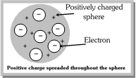
Thomson's model.
(1) Thomson regarded atom to be composed of positively charged protons and negatively charged electrons. The two types of particles are equal in number thereby making atom electrically neutral.
(2) He regarded the atom as a positively charged sphere in which negative electrons are uniformly distributed like the seeds in a water melon.
(3) This model failed to explain the line spectrum of an element and the scattering experiment of Rutherford.
(2) From the above observations he concluded more...
Dual Nature of Electron(1) In 1924, the french physicist, Louis de Broglie suggested that if light has both particle and wave like nature, the similar duality must be true for matter. Thus an electron, behaves both as a material particle and as a wave.(2) This presented a new wave mechanical theory of matter. According to this theory, small particles like electrons when in motion possess wave properties.(3) According to de-broglie, the wavelength associated with a particle of mass \[m,\] moving with velocity \[v\] is given by the relation \[\lambda \,=\,\frac{h}{mv},\] where h = Planck?s constant.(4) This can be derived as follows according to Planck?s equation, \[E=\,h\nu =\frac{h.c}{\lambda }\] \[\left( \because \ \ \nu =\frac{c}{\lambda } \right)\] energy of photon (on the basis of Einstein?s mass energy relationship), \[E=\,mc{}^{2}\] equating both \[\frac{hc}{\lambda }=\,\,mc{}^{2}\,\,or\,\,\lambda =\frac{h}{mc}\] which is same as de-Broglie relation. \[\left( \because \ \ mc=p \right)\](5) This was experimentally verified by Davisson and Germer by observing diffraction effects with an electron beam. Let the electron is accelerated with a potential of V than the Kinetic energy is \[\frac{1}{2}mv{}^{2}=\,\,eV\]; \[m{}^{2}v{}^{2}=\,\,2eVm\] \[mv=\sqrt{2eVm}=\,\,P\]; \[\lambda =\frac{h}{\sqrt{2eVm}}\](6) If Bohr?s theory is associated with de-Broglie?s equation then wave length of an electron can be determined in bohr?s orbit and relate it with circumference and multiply with a whole number \[2\pi r=n\lambda \,\,or\,\,\lambda =\frac{2\pi r}{n}\]From de-Broglie equation, \[\lambda =\frac{h}{mv}\]. Thus \[\frac{h}{mv}=\frac{2\pi r}{n}\] or \[mvr=\frac{nh}{2\pi }\] Note : qFor a proton, electron and an \[\alpha \]-particle moving with the same velocity have de-broglie wavelength in the following order : Electron > Proton > \[\alpha \]- particle.
(7) The de-Broglie equation is applicable to all material objects but it has significance only in case of microscopic particles. Since, we come across macroscopic objects in our everyday life, de-broglie relationship has no significance in everyday life.
Example: 34 An electron is moving with a kinetic energy of 4.55 × 10\[{}^{-25}\,\] J. What will be de-Broglie wavelength for this electron
(a) 5.28 × \[10{}^{-7}\,m\] (b) 7.28 × \[10{}^{-7}m\] (c) 2 × 10\[{}^{-10}m\] (d) 3 × \[10{}^{-5}m\]
Solution : (b) KE\[=\frac{1}{2}\,mv{}^{2}=\,4.55\,\,\times \,\,10{}^{-25}\] J
\[v{}^{2}=\frac{2\,\times 4.55\times 10{}^{-25}}{9.1\times 10{}^{-31}}=\,1\,\times \,10{}^{6}\]; \[v=10{}^{3}\,m/s\]
De-Broglie wavelength \[\lambda =\frac{h}{mv}=\frac{6.626\,\,\times \,\,10{}^{-34}}{9.1\,\times \,10{}^{-31}\times \,10{}^{3}}=\,\,7.28\,\,\times \,\,10{}^{-7}\,m\,\,\]
Example: 35 The speed of the proton is one more...
Uncertainty Principle and Schrodinger Wave Equation
Heisenberg’s uncertainty principle.
(1) One of the important consequences of the dual nature of an electron is the uncertainty principle, developed by Warner Heisenberg.
(2) According to uncertainty principle “It is impossible to specify at any given moment both the position and momentum (velocity) of an electron”.
Mathematically it is represented as, \[\Delta x\,.\,\Delta p\ge \frac{h}{4\pi }\]
Where \[\Delta x=\]uncertainty is position of the particle, \[\Delta p=\]uncertainty in the momentum of the particle
Now since \[\Delta p=m\,\Delta v\]
So equation becomes, \[\Delta x.\,m\Delta v\ge \frac{h}{4\pi }\] or \[\Delta x\,\times \,\Delta v\ge \frac{h}{4\pi m}\]
The sign \[\ge \] means that the product of \[\Delta x\]and \[\Delta p\](or of \[\Delta x\]and\[\Delta v\]) can be greater than, or equal to but never smaller than \[\frac{h}{4\pi }.\]If \[\Delta x\]is made small, \[\Delta p\]increases and vice versa.
(3) In terms of uncertainty in energy, \[\Delta E\]and uncertainty in time \[\Delta t,\]this principle is written as, \[\Delta E\,.\,\Delta t\ge \frac{h}{4\pi }\]
Note :q Heisenberg’s uncertainty principle cannot we apply to a stationary electron because its velocity is 0 and position can be measured accurately..
Example: 36 What is the maximum precision with which the momentum of an electron can be known if the uncertainty in the position of electron is \[\pm 0.001{\AA}?\] Will there be any problem in describing the momentum if it has a value of \[\frac{h}{2\pi {{a}_{0}}},\]where \[{{a}_{0}}\]is Bohr’s radius of first orbit, i.e., 0.529Å?
Solution : \[\Delta x\,.\,\Delta p=\frac{h}{4\pi }\]
\[\because \] \[\Delta x=0.001{\AA}={{10}^{-13}}m\]
\[\therefore \] \[\Delta p=\frac{6.625\times {{10}^{-34}}}{4\times 3.14\times {{10}^{-13}}}=5.27\times {{10}^{-22}}\]
Example: 37 Calculate the uncertainty in velocity of an electron if the uncertainty in its position is of the order of a 1Å.
Solution : According to Heisenberg’s uncertainty principle
\[\Delta v\,.\,\Delta x\approx \frac{h}{4\pi m}\]
\[\Delta v\approx \frac{h}{4\pi m.\Delta x}\] \[=\frac{6.625\times {{10}^{-34}}}{4\times \frac{22}{7}\times 9.108\times {{10}^{-31}}\times {{10}^{-10}}}\] \[=5.8\times {{10}^{5}}m\ \,{{\sec }^{-1}}\]
Example: 38 A dust particle having mass equal to \[{{10}^{-11}}g,\]diameter of \[{{10}^{-4}}cm\] and velocity \[{{10}^{-4}}cm\,{{\sec }^{-1}}.\]The error in measurement of velocity is 0.1%. Calculate uncertainty in its positions. Comment on the result.
Solution : \[\Delta v=\frac{0.1\times {{10}^{-4}}}{100}=1\times {{10}^{-7}}cm\,{{\sec }^{-1}}\]
\[\because \] \[\Delta v\,.\,\Delta x=\frac{h}{4\pi m}\]
\[\therefore \] \[\Delta x=\frac{6.625\times {{10}^{-27}}}{4\times 3.14\times {{10}^{-11}}\times 1\times {{10}^{-7}}}=5.27\times {{10}^{-10}}cm\]
The uncertainty in position as compared to particle size.
\[=\frac{\Delta x}{diameter}=\frac{5.27\times {{10}^{-10}}}{{{10}^{-4}}}=5.27\times {{10}^{-6}}cm\]
The factor being small and almost being negligible for microscope particles.
Schrödinger wave equation.
(1) Schrodinger wave equation is given by Erwin Schrödinger in 1926 and based on dual nature of electron.
(2) In it electron is described as a three dimensional wave in the electric field more...
Quantum Number, Electronic Configuration and Shape of Orbitals
Quantum numbers and Shapes of orbitals.
Quantum numbers
(1) Each orbital in an atom is specified by a set of three quantum numbers (n, l, m) and each electron is designated by a set of four quantum numbers (n, l, m and s).
(2) Principle quantum number (n)
(i) It was proposed by Bohr’s and denoted by ‘n’.
(ii) It determines the average distance between electron and nucleus, means it is denoted the size of atom.
\[r=\frac{{{n}^{2}}}{Z}\times 0.529{\AA}\]
(iii) It determine the energy of the electron in an orbit where electron is present.
\[E=-\frac{{{Z}^{2}}}{{{n}^{2}}}\times 313.3\,Kcal\,per\,mole\]
(iv) The maximum number of an electron in an orbit represented by this quantum number as \[2{{n}^{2}}.\] No energy shell in atoms of known elements possess more than 32 electrons.
(v) It gives the information of orbit K, L, M, N------------.
(vi) The value of energy increases with the increasing value of n.
(vii) It represents the major energy shell or orbit to which the electron belongs.
(viii) Angular momentum can also be calculated using principle quantum number
\[mvr=\frac{nh}{2\pi }\]
(3) Azimuthal quantum number (l)
(i) Azimuthal quantum number is also known as angular quantum number. Proposed by Sommerfield and denoted by ‘l’.
(ii) It determines the number of sub shells or sublevels to which the electron belongs.
(iii) It tells about the shape of subshells.
(iv) It also expresses the energies of subshells \[s<p<d<f\] (increasing energy).
(v) The value of \[l=(n-1)\] always where ‘n’ is the number of principle shell.
Important Terms And Classification Of AnimalsIntroduction and history of cellular enzymes.Enzymes (Gk. en = in; zyme = yeast) are proteinaceous substances which are capable of catalysing chemical reactions of biological origins without themselves undergoing any change. Enzymes are biocatalysts. An enzyme may be defined as "a protein that enhances the rate of biochemical reactions but does not affect the nature of final product." Like the catalyst the enzymes regulate the speed and specificity of a reaction, but unlike the catalyst they are produced by living cells only. All components of cell including cell wall and cell membrane have enzymes. Every cell produces its own enzymes because they can not move from cell to cell due to having high molecular weight. Maximum enzymes (70%) in the cell are found in mitochondrion. The study of the composition and function of the enzyme is known as enzymology.The term enzyme (meaning in yeast) was used by Willy Kuhne (1878) while working on fermentation. At that time living cells of yeast were thought to be essential for fermentation of sugar. Edward Buchner (1897), a German chemist proved that extract zymase, obtained from yeast cells, has the power of fermenting sugar (alcoholic fermentation). Zymase is complex of enzymes (Buchner isolated enzyme for the first time).Later J.B. Sumner (1926) prepared a pure crystalline form of urease enzyme from Jack Bean (Canavalia ensiformis) and suggested that enzymes are proteins. Northrop and Kunitz prepared crystals of pepsin, trypsin and chymotrpsin Arber and Nathans got noble prize in 1978 for the discovery of restriction endonucleases which break both strands of DNA at specific sites and produce sticky ends. These enzymes are used as microscissors in genetic engineering. Nature of enzymes.Mostly enzymes are proteinaceous in nature. With some exception all enzymes are proteins but all proteins are not enzymes. Enzymic protein consist of 20 amino acids, which constitute other proteins. More than 100 amino acids linked to form an active enzyme. The polypeptide chain or chains of an enzyme show tertiary structure. Sequence of the amino acid in specific enzymic proteins. Their tertiary structure is very specific and important for their biological activity. Loss of tertiary structure renders the enzyme activity.DNA is the master molecule, which contains genetic information for the synthesis of proteins. It has been found that DNA makes RNA and RNA finally makes proteins. The process of RNA formation from DNA template is known as transcription and synthesis of proteins as per information coded in mRNA is called translation. The above relation can be given by the more...
Classification and factors affecting enzymeNomenclature and Classification.
Dauclax, (1883) introduced the nomenclature of enzyme. Usually enzyme names end in suffix-ase to the name of substrate e.g. Lactase acts on lactose, maltase act on maltose, amylase on amylose, sucrase on sucrose, protease on proteins, lipase on lipids and cellulase on cellulose. Sometimes arbitrary names are also popular e.g. Pepsin, Trypsin and Ptylin etc. Few names have been assigned as the basis of the source from which they are extracted e.g. Papain from papaya, bromelain from pineapple (family Bromeliaceae). Enzymes can also be named by adding suffix?ase to the nature of chemical reaction also e.g. oxidase, dehydrogenase, catalase, DNA polymerase.
(1) According to order classification
The older classification of enzymes is based on the basis of reactions which they catalyse. Many earlier authors have classified enzymes into two groups:
(i) The hydrolysing enzymes
(ii) The desmolysing enzymes.
Other classify enzymes into three groups
(i) The hydrolysing enzymes
(ii) The transferring enzymes
(iii) The desmolysing enzymes
In the first classification transferring enzymes are included in the hydrolysing enzymes since some of them are known to act as transferring as well as hydrolysing enzymes.
(i) Hydrolysing enzyme: The hydrolysing enzymes of hydrolases catalyse reactions in which complex organic compounds are broken into simpler compounds with the addition of water. Most of the hydrolysing (digestive) enzymes are located in lysosomes. Depending upon the substrate hydrolysing enzymes are:
(a) Carbohydrases : Most of the polysaccharides, disccharides or small oligosaccharides are hydrolysed to simpler compounds, e.g., hexoses or pentoses under the influence of these enzymes.
Lactase on lactose to form glucose to galactose, sucrase/invertase on surcose to form glucose and fructose, amalyse or diastase on starch to form maltose, maltase on maltose to form glucose, cellulase on cellulose to produce glucose.
(b) Easterases : These enzymes catalyse the hydrolysis of substances containing easter linkage, e.g., fat, pectin, etc. into an alcoholic and an acidic compound.
\[\text{Fat}\xrightarrow{\text{lipase}}\text{Glycerol }+\text{ Fatty acid}\]
\[\text{Phosphoric acid easters }\xrightarrow{\text{phosphatase }}\text{Phosphoric acid }+\text{ Other compounds }\]
(c) Proteolytic enzymes : The hydrolysis of proteins into peptones, polypeptides and amino acids is catalysed by these enzymes
\[\text{Protein}\xrightarrow{\text{Pepsin}}\text{Peptones}\]
\[\text{Polypeptides}\xrightarrow{\text{Peptidases}}\text{Amino acids}\]
(d) Amidases : They hydrolyse amides into ammonia and acids.
\[\text{Urea}\xrightarrow{\text{Urease}}\text{Ammonia}+\text{Carbon dioxide}\]
\[\text{Asparagine}\xrightarrow{\text{asparaginase}}\text{Ammonia}+\text{Aspartic acid}\]
(ii) Desmolysing enzymes : Most of the desmolysing enzymes are the enzymes of respiration e.g. oxidases, dehydrogenases, (concerned with transfer of electrons), transaminases carboxylases etc.
(2) According to IUB system to classification
The number of enzymes is very large and there is much confusion in naming them. In 1961 the Commission on enzymes set up by the 'International Union of Biochemistry' (IUB) framed certain rules of their nomenclature and classification.
According to IUB system of classification the major points are :
· Reactions (and enzymes catalyzing them) are more...
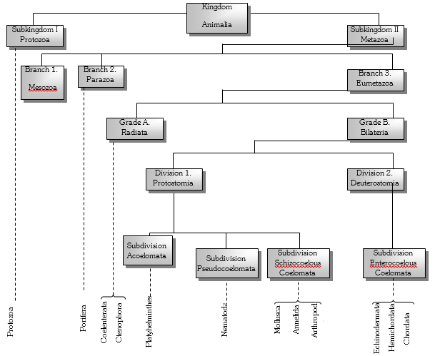
Important Terms And Classification Of AnimalsOutline Classification of Animal kingdom. The animal kingdom is subdivided into two sub-kingdoms, namely Protozoa and Metazoa. Subkingdom 1. Protozoa : It includes microscopic, unicellular animals. It contains a single Phylum called protozoa. e.g. Euglena, Amoeba, Paramecium etc.Subkingdom 2. Metazoa : This sub kingdom includes multicellular animals. e.g. Porifera to Chordata. The subkingdom Metazoa is divided into three branches, namely Mesozoa, Parazoa and Eumetazoa.Branch1. Mesozoa : It is intermediate between Protozoa and Metazoa. It includes endoparasitic animals. e.g. Dicyema, Rhopalura etc. Branch 2. Parazoa : It includes sponges. Branch 3. Eumetazoa : It includes true multicellular organisms. They have organ and organ system grade of organization. e.g. Coelenterata to Chordata. Eumetazoa is further divided into two grades, namely Radiata and Bilateria. Grade A. Radiata : It includes radially symmetrical animals. e.g. Coelenterata. Grade B. Bilateria : It includes bilaterally symmetrical animals. e.g. Platyhelminthes to Chordata The grade Bilateria is further divided into two divisions namely proterostomia and deuterostomia. Division 1. Proterostomia : In this group of animals, the blastopore develops into the mouth. e.g. It is further divided into 3 sub division.Sub division 1. Acoelomata: In this group more...
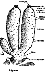
Phylum-PoriferaPhylum Porifera.(i)Introduction : Lowest multicellular animals or metazoans without true tissues, i.e., at ?Cellular level? of body organization. Familiar as sponges, these animals are well-known for their ability to absorb and withhold fluids. The word ?Porifera? means pore bearers (Gr., porus = pore; ferre = to bear); Their body wall has numerous minute pores, called ostia, through which a continuous current of outside water is drawn into the body. About 5,000 species are known.(ii)Brief History : Robert Grant (1825) finally proved that sponges are animals, and coined the name ?Porifera? for these. Schulze (1878), Butschli (1884), Sollas (1884) and Delage (1898) separated sponges from other metazoans on basis of embryological studies, and suggested a separate group, ?Parazoa? for these. (iii) Salient features : Phylum porifera has the following salient features :(1) All the sponges are Aquatic, Sedentary, Asymmetrical or Radially, First multicellular organisms and have cellular grade of organization.(2) They are diploblastic. Ectoderm is formed by pinachocyte and endoderm is formed by choanocyte. Both layers are called pinachoderm and choandoderm. (3) The body is perforated by numerous minute pores called ostia. (4) The ostia open into a large cavity called spongocoel. (5) The spongocoel opens to the outside by a large opening called osculum. (6) The sponges possess an endoskeleton in the form of calcareous spicules. (7) Excretion and respiration occur by diffusion. (8) They have greater power of regeneration. (9) Reproduction takes place by asexual or sexual more...
Phylum-Coelenterata Phylum Cnidaria (= Coelenterata).(i)Introduction : ?Tissue grade? eumetazoans with a radial symmetry. The term ?Coelenterata? signifies the presence of a single internal cavity called coelenteron, or gastrovascular cavity, combining functions of both digestive and body cavities. The term ?Cnidaria? indicates the presence of stinging cells (Gr., knide = nittle or stinging cells). About 9,000 species known.(ii)Brief History : Peyssonel (1723) and Trembley (1744) proved these to be animals. Hence, Linnaeus (1758), Cuvier (1796) and Lamarck (1801) included these under ?Zoophyta?, together with sponges. Leuckart (1847) included sponges and cnidarians under his phylum Coelenterata. Finally, Hatschek (1888) divided ?Coelenterata? into three phyla?Spongiaria (= Porifera), Cnidaria and Ctenophora. (iii)Salient Features : Phylum coelenterata has the following salient features ? (1) Coelenterates are multicellular organisms (2) They have tissue-grade of organization (3) The body is radially symmetrical. Radial symmetry is the symmetry of a wheel (4) All the members of this phylum are aquatic (5) They are solitary or colonial (6) Two types of individuals occur in the life cycle. They are polyps and medusa(7) The body wall is diploblastic. It is made up of two layers of cells, namely the ectoderm and the endoderm with a non?cellular layer called mesogloea in between. (8) Nematocysts or stinging cells are present (9) Coelom is absent; Hence coelenterates are acoelomate animals (10) A gastrovascular cavity or coelenteron is present. It can be compared to the gut of higher animals. more...
 Z= atomic number of the metal
\[a\And b\] are constant.
(iii) Atomic number = Number of positive charge on nucleus = Number of protons in nucleus = Number of electrons in nutral atom.
(iv) Two different elements can never have identical atomic number.
(2) Mass number
(i) The sum of proton and neutrons present in the nucleus is called mass number.
Mass number (A) = Number of protons + Number of neutrons or Atomic number (Z)
or Number of neutrons = A – Z .
(ii) Since mass of a proton or a neutron is not a whole number (on atomic weight scale), weight is not necessarily a whole number.
(iii) The atom of an element X having mass number (A) and atomic number (Z) may be represented by a symbol,
Z= atomic number of the metal
\[a\And b\] are constant.
(iii) Atomic number = Number of positive charge on nucleus = Number of protons in nucleus = Number of electrons in nutral atom.
(iv) Two different elements can never have identical atomic number.
(2) Mass number
(i) The sum of proton and neutrons present in the nucleus is called mass number.
Mass number (A) = Number of protons + Number of neutrons or Atomic number (Z)
or Number of neutrons = A – Z .
(ii) Since mass of a proton or a neutron is not a whole number (on atomic weight scale), weight is not necessarily a whole number.
(iii) The atom of an element X having mass number (A) and atomic number (Z) may be represented by a symbol,

 (2) From the above observations he concluded more...