Category : 10th Class
STATISTICS
INTRODUCTION
Data
The word ‘data’ means, information in the form of numerical figures or a set of given facts. For example, the percentage of marks scored by 10 students of a class in a test are: 36, 80, 65, 75, 94, 48, 12, 64, 88 and 98.
Row Data
Data obtained from direct observation is called raw data,
The marks obtained by 100 students in a. monthly test is an. example of raw data or ungrouped.
Intact, little can be inferred from this data. However, arranging the marks in ascending order in the above example is a step towards making raw data more meaningful.
Grouped Data
To present the data in a more meaningful way, we condense the data into convenient number of classes or groups, generally not exceeding 10 and not less than 5. This helps us in perceiving at a glance, certain salient features of data.
Tabulation or Presentation of Data
A systematically arrangement of the data in a tabular form is called ‘tabulation’ or ‘presentation’ of the data. This groping results in a table called ‘frequency table’ that indicates the number of scores within each group.
Individual Series: Any raw data that is collected, forms an individual series.
Example:
36, 35, 32, 40, 65, 48, 54, 71, 62 and 33
Discrete Series: A discrete series is formulated from raw data. Here, the frequency of the observations are taken into consideration.
Example: Given below is the data showing the number of computers in 15 families of a locality.
1, 1, 2, 3, 2, 1, 4, 3, 2, 2, 1, 1, 1, 1, 4
Arranging the data in ascending order:
1, 1, 1, 1, 1, 1, 1, 2, 2, 2, 2, 3, 3, 4, 4
To count, we can use tally marks. We record tally marks in bunches of five, the fifth one crossing the other four diagonally, i.e.
Thus, we may prepare the following frequency table.
|
Number of Computers |
Tally Marks |
Number of Families (Frequency) |
|
1 |
\[\cancel{IIII}II\] |
7 |
|
2 |
\[IIII\] |
4 |
|
3 |
\[II\] |
2 |
|
4 |
\[II\] |
2 |
Continuous Series: When the data contains large number of observation, we put them into different groups called ‘class intervals’. Such as 1 – 10, 11 – 20, 21 – 30, 31 – 40, 41 – 50 etc…… Here, 1 – 10 means data whose values lies between 1 and 10 including both 1 and 10.
Class interval
A group into which the raw data is condensed is called a class interval.
Each class is bounded by two figures which are called the class limits. The figure on the LHS is called lower limit and. the figure on the RHS is called upper limit of the class. Thus. 0 – 10 is a class with lower limit being ‘O’ and the upper limit being ‘10’.
Class size
The difference between the true upper limit and the true lower limit is called ‘class size’.
Class interval 15 – 25 the class size = 25 – 15 = 10.
Class Mark or Mid value
Class mark \[=\frac{1}{2}\] (upper limit + lower limit)
Thus, the class mark of 15 – 25 is: \[\frac{1}{2}\] (25 + 15) = 20.
Methods of finding the mean of a grouped data: Mean of a grouped data is calculated using (a) Direct method (b) Assumed mean method and (c) Step deviation method.
(a) Direct method: If the observations \[{{x}_{1}},{{x}_{2}},......,{{x}_{n}}\] appear with frequencies, \[{{f}_{1}},{{f}_{21}},......,{{f}_{n}}\], then mean is given by \[x=\frac{1}{N}\sum\limits_{i=1}^{n}{{{f}_{1}}{{x}_{1}}}\], where \[N={{f}_{1}}+{{f}_{2}}+.......+{{f}_{n}}\].
(b) Assumed mean method: In this method, we choose an assumed mean ‘a’ and subtract it from each of the values\[{{x}_{i}}\]. The reduced value \[{{x}_{i}}-a\] is called the deviation of x, from ‘a’. The deviations are then multiplied by corresponding frequencies to get fi di. Then the sum of \[{{f}_{i}}{{d}_{i}}\] is computed.
Arithmetic mean =\[a+\frac{\sum\limits_{i=1}^{n}{{{f}_{i}}{{d}_{i}}}}{\sum\limits_{i=1}^{n}{{{f}_{i}}}}\]
Note: The assumed mean is chosen in such a way that it is one of the central values, the deviations are small and one of the deviations is zero.
(c) Step deviation method: The deviation method is further simplified on dividing the deviation by width of the class interval h. Then arithmetic mean \[_{x}^{-}=a+\frac{\sum{{{f}_{i}}{{u}_{i}}}}{\sum{{{f}_{i}}}}\times h\]
Where \[{{u}_{i}}=\frac{{{x}_{i}}-a}{h}.\]
MEDIAN
Another measure of central tendency of a given data is the median.
Concept of Median:
Properties of Mode
Relationship between mean, median, mode
Mean – Mode = 3 (Mean – Median): Hence, given any two of the mean, median and mode, the third quantity can be calculated.
Mode
Formula for calculating median: Median \[(M)=L+\frac{\frac{n}{2}-{{C}_{f}}}{f}(C)\]
Where, L = Lower boundary of the median class i.e., class in which \[\left( \frac{n}{2} \right)th\] observation lies.
n = Sum of frequencies
\[{{C}_{f}}=\] cumulative frequency of the class just preceding the median class
f = frequency of median class
C = length of class interval
Mode of Grouped Data
The formula for determining the mode of grouped data is \[{{L}_{1}}+\frac{{{\Delta }_{1}}C}{{{\Delta }_{1}}+{{\Delta }_{2}}}\] ............... (i)
Where, \[{{L}_{1}}=\] lower boundary of modal class (class with highest frequency).
\[{{\Delta }_{1}}=f-{{f}_{1}}\]and \[{{\Delta }_{2}}=f-{{f}_{2}}\], where f is the frequency of modal class
\[{{f}_{1}}=\] frequency of the previous class to the modal class
\[{{f}_{2}}=\] frequency of the next class of the modal class.
The formula for mode can also be written as:
\[\text{Mode}={{L}_{1}}+\frac{(f-{{f}_{1}})C}{(f-{{f}_{1}})+(f-{{f}_{2}})}\] ……………….(ii)
Variance =\[{{(SD)}^{2}}\], or \[SD=\sqrt{\operatorname{variance}}\]
\[SD(\sigma )=\sqrt{\frac{{{\left( {{x}_{1}}-\overline{x} \right)}^{2}}+{{\left( {{x}_{2}}-\overline{x} \right)}^{2}}+.....+{{\left( {{x}_{n}}-\overline{x} \right)}^{2}}}{n}}=\sqrt{\frac{\sum\limits_{i=1}^{n}{{{\left( {{x}_{i}}-\overline{x} \right)}^{2}}}}{n}}\]
Where, \[{{x}_{1}},{{x}_{2}}.......,{{x}_{n}}\]are n observation and their mean is \[\overline{x}\]
QUARTILES
The observations that divide the given set of observations into four equal parts are called Quartiles.
First Quartile or Lower Quartile
When the given observations are arranged in ascending order, the observation which lies midway between the lower extreme and the median is called the first quartile, or the lower quartile, and is denoted as\[{{Q}_{1}}\].
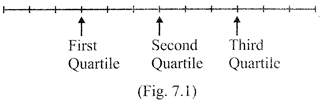
First quartile second quartile Third quartile
Second quartile is actually median (for Raw / Individual data) looking at figure above (figure.7.1), you will find that if 12 observations are arranged in ascending order. Then third observation is first (or lower) quartile\[\left( 3=\frac{1}{4}\times 12 \right)\]; sixth observation is second quartile (or median)\[\left( \text{since},6=\frac{1}{2}\times 12 \right)\] Whereas, ninth observation is Third (or upper) Quartile
\[\left( \text{since},9=\frac{3}{4}\times 12 \right)\].


You need to login to perform this action.
You will be redirected in
3 sec

