Control System
Category : Railways
Control System
CONTROL SYSTEM
It is an arrangement of different physical components in such a way that we get the desired output from the input.
Classification of Control System
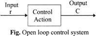
For example: traffic light, tap of water etc.
Advantages: These systems are simple in construction & design; economic in nature; easy from the maintenance point of view, have high stability & are convenient to use when the output is difficult to measure.
Disadvantages: These systems are not accurate & reliable as the accuracy depends on the calibration of the inputs & their operation is affected due to the presence of non-linearities in the elements.
For example A. C., humans etc.
Advantages: These systems have high accuracy: system errors can be modified as these systems can sense environmental changes as well as internal disturbances. They also have less reduced effects of non-linearities, and have high bandwidth
Disadvantages: These systems are complicated to construct, and are costly & unstable in nature.
PRINCIPLE OF FEEDBACK
In the open loop system, there is no feedback path, but this feedback path exists in a closed loop system. So, in a closed loop system, the output will also depend on the feedback system. The purpose of feedback is to reduce the error which exists due to the difference in reference input and system output.
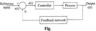
There are two types of feedback:
1) Positive feedback
2) Negative feedback
Positive feedback: When the output which is fed as an input to the system, is in the same phase with the input, then this feedback increases the input or it is added to the input. The positive feedback is used in oscillator circuits.
For positive feedback, error signal \[=r(t)+c(t)\]

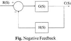
Negative feedback: When the output which is fed as an input to the system, is in a completely opposite phase to the input, then this feedback reduces the input or is subtracted from the input. This feedback helps in stabilizing the gain of the amplifier. Negative feedback is used in amplifier circuits.
For negative feedback, error signal =r (t) - c (t)
Effects of Feedback:
BLOCK DIAGRAM REDUDCTION TECHNIQUES:
|
Manipulation |
Original Block diagram |
Equivalent Block diagram |
Equation |
|
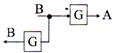
Blocks in cacade |
|
|
\[A=({{G}_{1}}{{G}_{2}})B\] |
|
Blocks in parallel |
|
|
\[A=({{G}_{1}}+{{G}_{2}})B\] |
|
Shifting take-off point at the back of the block |
|
|
\[A=GB\,\,or\,\,B\,=A/G\] |
|
Shifting take-off point at the front of the block |
|
|
\[A=GB\] |
|
Shifting summing point at the front of the block |
|
|
\[A=G{{B}_{1}}-{{B}_{2}}\] |
|
Shifting summing point at the back of the block |
|
|
\[{{E}_{2}}=G({{B}_{1}}-{{B}_{2}})\] |
Rules for Drawing SFG
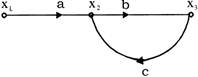
Signal flow graph with one forward path and single isolated loop Fig.
At node \[{{x}_{2}},{{x}_{2}}=a{{x}_{1}}+c{{x}_{3}}\]
At node \[{{x}_{3}},{{x}_{3}}=b{{x}_{2}}\]
TRANSFER FUNCTIONS
\[G(s)=\frac{C(s)}{R(s)}\,\,or\,\,C(s)=G(s)R(s)\]

Fig.
Suppose a transfer function of a linear control system is given by
\[G(s)=\frac{A(s)}{B(s)}=\frac{K(s-{{s}_{1}})(s-{{s}_{2}})(s-{{s}_{3}})....(s-{{s}_{n}})}{(s-{{s}_{a}})(s-{{s}_{b}})(s-{{s}_{c}})....(s-{{s}_{m}})}\]
where 'K' is the gain factor of transfer function.
Poles of transfer function: In above expression, ifs is put equal to\[{{s}_{a}},\,\,{{s}_{b}},\,\,{{s}_{c}}.....{{s}_{m}},\], then it is observed that the value of transfer function becomes infinite, thus\[{{s}_{a}},\,\,{{s}_{b}},\,\,{{s}_{c}}.....{{s}_{m}},\] are called poles of the transfer function; it is represented by X.
Zeros of transfer function: In above expression, ifs is put equal to\[{{s}_{1}},\,\,{{s}_{2}},\,\,{{s}_{3}}.....{{s}_{n}},\], then it is observed that the value of transfer function becomes zero, thus\[{{s}_{1}},\,\,{{s}_{2}},\,\,{{s}_{3}}.....{{s}_{n}},\]are called zeros of the transfer function; it is represented by 0.
For \[s=\infty \]
STEADY STATE ERRORS
G (s) H (s) of the system, which is given by
\[G\,\,(s)H\,\,(s)=\frac{K\,\,(1+s{{T}_{a}})\,\,(1+s{{T}_{b}}).....}{{{s}^{N}}(1+{{s}^{T}}_{1})\,\,(1+s{{T}_{2}})....}\]
where K is the forward path gain, N is the number of poles at the origin and
\[\left. \begin{matrix}
-\frac{1}{{{T}_{a}}},\,\,-\frac{1}{{{T}_{b}}}......are\,\,zeros \\
-\frac{1}{{{T}_{1}}},\,\,-\frac{1}{{{T}_{2}}}......are\,\,poles \\
\end{matrix} \right\}\]
When N = N, system is called as type N system.

\[\frac{E\,\,(s)}{R\,\,(s)}=\frac{1}{1+G\,\,(s)\,\,H\,\,(s)}\]
If \[f(t)\xrightarrow{laplace\,\,transform}F\,\,(s)\]
then \[\underset{t\to \infty }{\mathop{lim}}\,\,\,f(t)=\underset{s\to 0}{\mathop{lim}}\,F(s)\]
\[{{e}_{ss}}=\underset{s\to 0}{\mathop{\lim }}\,\,\,sE(s)\,\,\underset{s\to 0}{\mathop{lim}}\,\,\,sR(s).\frac{1}{1+G(s)\,\,H(s)}\]
TECHNIQUES USED TO CALCULATE STABILITY
Routh–Hurwitz Criterion
NYQUIST PATH OR NYQUIST CONTOUR
The overall transfer of a system is given by.
\[\frac{C(s)}{R(s)}=\frac{G(s)}{1+G(s)\,\,H(s)}\]
The characteristic equation is 1 + G(s) H(s) = 0
The main purpose in study the stability of the closed loop system is to determine whether the characteristic equation has any root in the right half of s-plane i.e. whether C(s)/R(s) has any pole in right half of s-plane.
For this purpose, we use a contour in s-plane which encloses the entire right half plane. This contour having the encirclement in clockwise direction and radius 'R' approaches infinity. This path or contour is known as Nyquist contour shown in fig. (a) If the system does not have any pole or zero at origin then the contour is shown in fig. (b).

GENERAL CONSTRUCTION RULES OF THE NYQUIST PATH
Consider the fig.
|
Path ab |
\[s=j\omega \,\,0<\omega <{{\omega }_{0}}\] |
(i) |
|
Path bc |
\[s=\underset{p\to 0}{\mathop{lime\,\,}}\,(j{{\omega }_{0}}+P{{e}^{j\theta }})-90{}^\circ \le \theta \le 90{}^\circ \] |
(ii) |
|
Path cd |
\[s=j\omega \,\,{{\omega }_{0}}\le \omega \le \infty \] |
(iii) |
|
Path def |
\[s=\underset{R\to \infty }{\mathop{lim}}\,{{\operatorname{Re}}^{j\theta }}-90{}^\circ \le \theta \le 90{}^\circ \] |
(iv) |
|
Path fg |
\[s=j\omega -\infty <\omega <-{{\omega }_{0}}\] |
(v) |
|
Path gh |
\[s=\underset{P\to 0}{\mathop{\lim \,\,}}\,(J{{\omega }_{0}}+P{{e}^{j\theta }})-90{}^\circ \le \theta \le 90{}^\circ \] |
(vi) |
|
Path hi |
\[s=j\omega \,\,{{\omega }_{0}}\le \omega \le 0\] |
(vii) |
|
Path ija |
\[s=\underset{P\to 0}{\mathop{lim}}\,P{{e}^{j\theta }}-90{}^\circ \le \theta \le 90{}^\circ \] |
(viii) |
Step 1: Check G(s) for poles on\[j\omega \]axis and at the origin
Step 2: Using \[e{{q}^{n}}\](i) to \[e{{q}^{n}}\](iii) sketch the image of the path \[a-d\]in the \[G\left( s \right)-\]plane. If there are no poles on\[j\omega \]axis equation (ii) need not be employed.
Step 3: Draw the mirror image about the real axis of the sketch resulting from step 2.
Step 4: Use \[e{{q}^{n}}\](iv) plot the image of path def. This path at infinity usually plot into a point in the \[G\left( s \right)-\]plane.
Step 5: Use \[e{{q}^{n}}\](viii) plot the image of path ija (pole at origin)
Step 6: Connect all curves drawn into the previous steps.
BODE PLOT
& a closed loop system. It is also called comer plot & asymptotic plot.
\[G.M.=20\,\,{{\log }_{10}}\frac{1}{|G\,\,(J{{\omega }_{2}})\,\,H\,\,(j{{\omega }_{2}})|}\]
Where\[{{\omega }_{2}}\]of is the phase cross frequency where \[\angle G\,\,(j\omega )\,\,H\,\,(j\omega ){}^\circ \] line crosses the frequency axis.
\[P.M.=180{}^\circ +\angle G\,\,(j{{\omega }_{1}})\,\,H\,\,(j{{\omega }_{1}}){}^\circ \]
Where \[\angle G\,\,(j{{\omega }_{1}})\,\,H\,\,(j{{\omega }_{1}}){}^\circ \]is measured clockwise & \[{{\omega }_{1}}\]is the gain crossover frequency at which\[|G\,\,(j\omega )\,\,H\,\,(j\omega )\,\,H\,\,(j\omega )|\]crosses the frequency axis.
ROOT LOCUS
State Transistion Matrix
It is a matrix which statistics the linear homogeneous state equation.
It is given by\[\phi \,\,(t)={{L}_{-1}}[{{(sI-A)}^{-1}}]\]& is of the order: n\[\times \]n.
Properties of state transistion matrix:
CONTROLLABILITY OF LINEAR CONTROL SYSTEM
It is in relation to the transfer of a system from one state to another by appropriate input controls in a finite time.
For the system to be completely controllable, it is sufficient that the n\[\times \]nr matrix has a rank of n.
\[U=[B:AB:{{A}^{2}}B....{{A}^{n-1}}B]\]
Where U = Controllability test matrix which is n \[\times \] nr.
OBSERVABILITY OF LINEAR CONTROL SYSTEM:
\[n~\times np\]row matrix form & is given by
\[V=[{{C}^{T}}:{{A}^{T}}{{C}^{T}}:{{({{A}^{T}})}^{2}}{{C}^{T}}:....{{({{A}^{T}})}^{n-1}}{{C}^{T}}]\]
And controlling torque, \[{{T}_{c}}={{K}_{c}}\theta \]
At steady position of pointer, \[{{T}_{c}}={{T}_{d}}\]
And thus, \[\theta \propto {{I}^{2}}\]
The transfer function is in the form:
\[G\,\,(s)=\frac{K\omega _{n}^{2}}{{{s}^{2}}+2\xi {{\omega }_{n}}s+\omega _{n}^{2}},\] \[\xi >0{{\omega }_{n}}>0\]
Here, K is called the DC gain, \[{{\omega }_{n}}\]is called the natural frequency, and\[\xi \]is called the damping ratio of the system. We will consider three case:
Case 1: \[\xi >1\]
This case is called the overdamped case.
\[{{\omega }_{d}}={{\omega }_{n}}\,\,\left( \xi -\sqrt{{{\xi }^{2}}-1} \right)\]
Case 2: \[\xi =1\]
This case is called the critically damped case.
Case 3: \[0<\xi <1\]
This case is called the underdamped case.
Maximum percent overshoot
\[{{M}_{P}}={{e}^{\frac{-\xi \pi }{\sqrt{1-{{\xi }^{2}}}}}}\]


You need to login to perform this action.
You will be redirected in
3 sec