JEE Main & Advanced Physics Electrostatics & Capacitance Electric Field and Potential Due to Various Charge Distribution

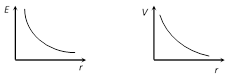
(1) Point charge : Electric field and potential at point P due to a point charge Q is

\[E=k\frac{Q}{{{r}^{2}}}\,\,\,\text{or}\,\,\,\vec{E}=k\frac{Q}{{{r}^{2}}}\hat{r}\]  \[\left( k=\frac{1}{4\pi {{\varepsilon }_{0}}} \right)\],   \[V=k\frac{Q}{r}\]

Graph

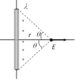
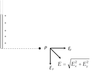
(2) Line charge: Electric field and potential due to a charged straight conducting wire of length \[l\] and charge density\[\lambda \] 

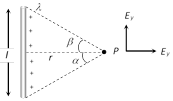
\[{{E}_{x}}=\frac{k\lambda }{r}(\sin \alpha +\sin \beta )\] and \[{{E}_{y}}=\frac{k\lambda }{r}(\cos \beta -\cos \alpha )\]

\[V=\frac{\lambda }{2\pi {{\varepsilon }_{0}}}{{\log }_{e}}\,\left[ \frac{\sqrt{{{r}^{2}}+{{l}^{2}}}-l}{\sqrt{{{r}^{2}}+{{l}^{2}}}+l} \right]\]

(i) If point P lies at perpendicular bisector of wire i.e. \[\alpha =\beta ;\,\,{{E}_{x}}=\frac{2k\lambda }{r}\sin \alpha \] and \[{{E}_{y}}=0\]

(ii) If wire is infinitely long i.e. \[l\to \infty \] so \[\alpha =\beta =\frac{\pi }{2};\,{{E}_{x}}=\frac{2k\lambda }{r}\] and \[{{E}_{y}}=0\Rightarrow {{E}_{net}}=\frac{\lambda }{2\pi {{\varepsilon }_{0}}r}\] and \[V=\frac{-\lambda }{2\pi {{\varepsilon }_{0}}}{{\log }_{e}}r+c\]

(iii) If point P lies near one end of infinitely long wire i.e.  \[\alpha =0,\,\] and \[\beta =\frac{\pi }{2}\]

\[|{{E}_{x}}|\,=\,|{{E}_{y}}|\,=\frac{k\lambda }{r}\]

\[\Rightarrow \] \[{{E}_{net}}=\sqrt{E_{x}^{2}+E_{y}^{2}}=\frac{\sqrt{2}\,k\lambda }{r}\]

(3) Charged circular ring : Suppose we have a charged circular ring of radius R and charge Q. On it's axis electric field and potential is to be determined, at a point 'x' distance away from the centre of the ring.

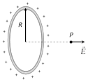
At point P

\[E=\frac{k\,Q\,x}{{{({{x}^{2}}+{{R}^{2}})}^{3/2}}},\]\[V=\frac{k\,Q}{\sqrt{{{x}^{2}}+{{R}^{2}}}}\]  

At centre \[x=0\] so \[{{E}_{centre}}=0\] and \[{{V}_{centre}}=\frac{kQ}{R}\]

At a point on the axis such that \[x>>R\] \[E=\frac{kQ}{{{x}^{2}}}\], \[V=\frac{kQ}{x}\]

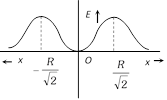
If  \[x=\pm \frac{R}{\sqrt{2}}\], \[{{E}_{\max }}=\frac{Q}{6\sqrt{3}\pi {{\varepsilon }_{0}}{{a}^{2}}}\] and  \[{{V}_{\max }}=\frac{Q}{2\sqrt{6}\pi {{\varepsilon }_{0}}}\]  

Graph

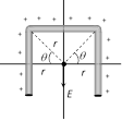
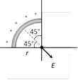
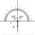
(4) Some more results of line charge : If a thin plastic rod having charge density \[\lambda \]  is bent in the following shapes then electric field at P in different situations shown in the following table     Bending of charged rod  

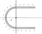
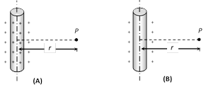
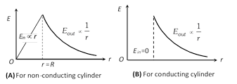
(5) Charged cylinder

(i) Non-conducting uniformly charged cylinder	(ii) Conducting charged cylinder

If point of observation (P) lies outside the cylinder then for both type of cylindrical charge distribution \[{{E}_{out}}=\frac{\lambda }{2\pi {{\varepsilon }_{0}}r}\], and \[{{V}_{out}}=\frac{-\lambda }{2\pi {{\varepsilon }_{0}}}{{\log }_{e}}r+c\]

If point of observation lies at surface i.e. \[r=R\] so for both cylinder \[{{E}_{suface}}=\frac{\lambda }{2\pi {{\varepsilon }_{0}}R}\] and \[{{V}_{surface}}=\frac{-\lambda }{2\pi {{\varepsilon }_{0}}}{{\log }_{e}}R+c\]

If point of observation lies inside the cylinder then for conducting cylinder \[{{E}_{in}}=0\] and for non-conducting \[{{E}_{\text{in}}}=\frac{\lambda r}{2\pi {{\varepsilon }_{0}}{{R}^{2}}}\]

Graph

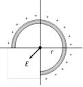
(6) Charged Conducting sphere (or shell of charge) : If charge on a conducting sphere of radius R is Q (and \[\sigma =\] surface charge density) as shown in figure then electric field and potential in different situation are

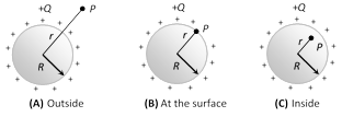
(i) Out side the sphere : If point P lies outside the sphere

\[{{E}_{out}}=\frac{1}{4\pi {{\varepsilon }_{0}}}.\frac{Q}{{{r}^{2}}}=\frac{\sigma {{R}^{2}}}{{{\varepsilon }_{0}}{{r}^{2}}}\] and \[{{V}_{out}}=\frac{1}{4\pi {{\varepsilon }_{0}}}.\frac{Q}{r}=\frac{\sigma {{R}^{2}}}{{{\varepsilon }_{0}}r}\] \[(Q=\sigma \times A=\sigma \times 4\,\pi {{R}^{2}})\]  

(ii) At the surface of sphere : At surface \[r=R\]

So, \[{{E}_{s}}=\frac{1}{4\pi {{\varepsilon }_{0}}}.\frac{Q}{{{R}^{2}}}=\frac{\sigma }{{{\varepsilon }_{0}}}\] and \[{{V}_{s}}=\frac{1}{4\pi {{\varepsilon }_{0}}}.\frac{Q}{R}=\frac{\sigma R}{{{\varepsilon }_{0}}}\]

(iii) Inside the sphere : Inside the conducting charge sphere electric field is zero and potential remains constant every where and equals to the potential at the surface.        

\[{{E}_{in}}=0\] and \[{{V}_{in}}\]= constant \[={{V}_{s}}\]

Graph

(7) Uniformly charged non-conducting sphere : Suppose charge Q is uniformly distributed in the volume of a non-conducting sphare of radius R as shown below 

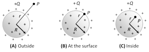
(i) Outside the sphere : If point P lies outside the sphere         

\[{{E}_{out}}=\frac{1}{4\pi {{\varepsilon }_{0}}}.\frac{Q}{{{r}^{2}}}\] and \[{{V}_{out}}=\frac{1}{4\pi {{\varepsilon }_{0}}}.\frac{Q}{r}\]

If the sphere has uniform volume charge density \[\rho =\frac{Q}{\frac{4}{3}\pi {{R}^{3}}}\]

then\[{{E}_{out}}=\frac{\rho {{R}^{3}}}{3{{\varepsilon }_{0}}{{r}^{2}}}\] and \[{{V}_{out}}=\frac{\rho {{R}^{3}}}{3{{\varepsilon }_{0}}r}\]

(ii) At the surface of sphere : At surface \[r=R\]        

\[{{E}_{s}}=\frac{1}{4\pi {{\varepsilon }_{0}}}.\frac{Q}{{{R}^{2}}}=\frac{\rho R}{3{{\varepsilon }_{0}}}\] 

and     \[{{V}_{s}}=\frac{1}{4\pi {{\varepsilon }_{0}}}.\frac{Q}{R}=\frac{\rho {{R}^{2}}}{3{{\varepsilon }_{0}}}\]

(iii) Inside the sphere : At a distance r from the centre        

\[{{E}_{in}}=\frac{1}{4\pi {{\varepsilon }_{0}}}.\frac{Qr}{{{R}^{3}}}\] \[=\frac{\rho r}{3{{\varepsilon }_{0}}}\] \[\left\{ {{E}_{in}}\propto r \right\}\]

and \[{{V}_{in}}=\frac{1}{4\pi {{\varepsilon }_{0}}}\frac{Q\,[3{{R}^{2}}-{{r}^{2}}]}{2{{R}^{3}}}=\frac{\rho (3{{R}^{2}}-{{r}^{2}})}{6{{\varepsilon }_{0}}}\]

At centre \[r=0\]  so, \[{{V}_{\text{centre}}}=\frac{3}{2}\times \frac{1}{4\pi {{\varepsilon }_{0}}}.\frac{Q}{R}=\frac{3}{2}{{V}_{s}}\]

i.e.,   \[{{V}_{centre}}>{{V}_{surface}}>{{V}_{out}}\]

Graph

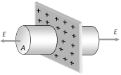
(8) Infinite thin plane sheet of charge : Consider a thin infinite non-conducting plane sheet having uniform surface charge density is \[\sigma \] . Electric field and potential near the sheet are

as follows \[E=\frac{\sigma }{2{{\varepsilon }_{0}}}\,\,\,\,(E\propto {{r}^{o}})\]

and \[V=-\frac{\sigma \,r}{2{{\varepsilon }_{0}}}+C\]

(9) Electric field due to two thin infinite plane parallel sheet of charge : Consider two large, uniformly charged parallel. Plates A and B, having surface charge densities are \[{{\sigma }_{A}}\] and \[{{\sigma }_{B}}\] respectively. Suppose net electric field at points P, Q and R is to be calculated.

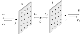
At P,  \[{{E}_{P}}=-({{E}_{A}}+{{E}_{B}})=-\frac{1}{2{{\varepsilon }_{0}}}({{\sigma }_{A}}+{{\sigma }_{B}})\]

At Q, \[{{E}_{Q}}=({{E}_{A}}-{{E}_{B}})=\frac{1}{2{{\varepsilon }_{0}}}({{\sigma }_{A}}-{{\sigma }_{B}})\]

At R, \[{{E}_{R}}=({{E}_{A}}+{{E}_{B}})=\frac{1}{2{{\varepsilon }_{0}}}({{\sigma }_{A}}+{{\sigma }_{B}})\]

Special cases  

(i) If \[{{\sigma }_{A}}={{\sigma }_{B}}=\sigma \] then \[{{E}_{P}}={{E}_{R}}=\sigma /{{\varepsilon }_{0}}\] and \[{{E}_{q}}=0\]

(ii) If \[{{\sigma }_{A}}=\sigma \] and \[{{\sigma }_{B}}=-\sigma \] then \[{{E}_{P}}={{E}_{R}}=0\] and \[{{E}_{Q}}=\sigma /{{\varepsilon }_{0}}\]

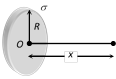
(10) Hemispherical charged body

At centre O,    \[E=\frac{\sigma }{4{{\varepsilon }_{0}}}\]

\[V=\frac{\sigma R}{2{{\varepsilon }_{0}}}\]

(11) Uniformly charged disc : At a distance \[x\] from centre O on it's axis

\[E=\frac{\sigma }{2{{\varepsilon }_{0}}}\left[ 1-\frac{x}{\sqrt{{{x}^{2}}+{{R}^{2}}}} \right]\]  

\[V=\frac{\sigma }{2{{\varepsilon }_{0}}}\left[ \sqrt{{{x}^{2}}+{{R}^{2}}}-x \right]\]

If \[x\to 0,\] \[E\tilde{}\,\frac{\sigma }{2{{\varepsilon }_{0}}}\] i.e. for points situated near the disc, it behaves as an infinite sheet of charge.