Kinds of function
Category : JEE Main & Advanced
(1) One-one function (injection) : A function \[f:A\to B\] is said to be a one-one function or an injection, if different elements of A have different images in B. Thus, \[f:A\to B\] is one-one.
\[a\ne b\,\,\Rightarrow \,\,f(a)\ne f(b)\] for all \[a,\,\,b\in A\]
\[\Leftrightarrow \,\,f(a)=f(b)\,\,\Rightarrow \,\,a=b\] for all \[a,\,\,b\in A\].
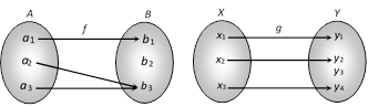
e.g. Let \[f:A\to B\] and \[g:X\to Y\] be two functions represented by the following diagrams.
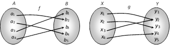
Clearly, \[f:A\to B\] is a one-one function. But \[g:X\to Y\] is not one-one function because two distinct elements \[{{x}_{1}}\] and \[{{x}_{3}}\] have the same image under function \[g\].
(i) Method to check the injectivity of a function
Step I : Take two arbitrary elements \[x,\,\,y\] (say) in the domain of \[f\].
Step II : Put \[f(x)=f(y).\]
Step III : Solve \[f(x)=f(y).\] If \[f(x)=f(y)\] gives \[x=y\] only, then \[f:A\to B\] is a one-one function (or an injection). Otherwise not.
If function is given in the form of ordered pairs and if two ordered pairs do not have same second element then function is one-one.
If the graph of the function \[y=f(x)\] is given and each line parallel to x-axis cuts the given curve at maximum one point then function is one-one. e.g.
(ii) Number of one-one functions (injections) : If \[A\] and \[B\] are finite sets having \[m\] and \[n\] elements respectively, then number of one-one functions from \[A\] to \[B\]\[=\left\{ \begin{align} & ^{n}{{P}_{m}},\,\,\,\text{if }n\ge m \\ & \,\,0\,\,\,\,,\,\,\,\text{if }n
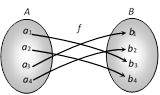
· If function is given in the form of set of ordered pairs and the second element of atleast two ordered pairs are same then function is many-one.
· If the graph of \[y=f(x)\] is given and the line parallel to x-axis cuts the curve at more than one point then function is many-one.
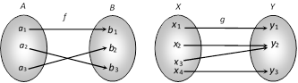
(3) Onto function (surjection) : A function \[f:A\to B\] is onto if each element of B has its pre-image in A. Therefore, if \[{{f}^{-1}}(y)\in A,\,\,\forall y\in B\] then function is onto. In other words, Range of \[f=\] Co-domain of f. e.g. The following arrow-diagram shows onto function.
Number of onto function (surjection) : If A and B are two sets having \[m\] and \[n\] elements respectively such that \[1\le n\le m,\] then number of onto functions from A to B is \[\sum\limits_{r=1}^{n}{{{(-1)}^{n-r}}{{\,}^{n}}{{C}_{r}}{{r}^{m}}.}\]
(4) Into function : A function \[f:A\to B\] is an into function if there exists an element in B having no pre-image in A.
In other words, \[f:A\to B\] is an into function if it is not an onto function e.g. The following arrow-diagram shows into function.
(i) Method to find onto or into function
(a) Solve \[f(x)=y\] by taking \[x\] as a function of\[y\] i.e., \[g(y)\] (say).
(b) Now if \[g(y)\] is defined for each \[y\in \]co-domain and \[g(y)\in \] domain for \[y\in \] co-domain, then \[f(x)\] is onto and if any one of the above requirements is not fulfilled, then \[f(x)\] is into.
(5) One-one onto function (bijection) : A function \[f:A\to B\] is a bijection if it is one-one as well as onto.
In other words, a function \[f:A\to B\] is a bijection if
(i) It is one-one i.e., \[f(x)=f(y)\,\Rightarrow \,\,x=y\]for all \[x,\,\,y\in A.\]
(ii) It is onto i.e., for all \[y\in B\], there exists \[x\in A\] such that \[f(x)=y.\]
Clearly, f is a bijection since it is both injective as well as surjective.
Number of one-one onto function (bijection) : If A and B are finite sets and \[f:A\to B\] is a bijection, then A and B have the same number of elements. If A has n elements, then the number of bijection from A to B is the total number of arrangements of n items taken all at a time i.e. \[n!\].
(6) Algebraic functions : Functions consisting of finite number of terms involving powers and roots of the independent variable and the four fundamental operations \[+,\,-,\,\,\times \] and \[\div \] are called algebraic functions.
e.g., (i) \[{{x}^{\frac{3}{2}}}+5x\]
(ii) \[\frac{\sqrt{x+1}}{x-1},\,x\ne 1\]
(iii) \[3{{x}^{4}}-5x+7\]
(7) Transcendental function : A function which is not algebraic is called a transcendental function. e.g., trigonometric; inverse trigonometric , exponential and logarithmic functions are all transcendental functions.
(i) Trigonometric functions : A function is said to be a trigonometric function if it involves circular functions (sine, cosine, tangent, cotangent, secant, cosecant) of variable angles.
(a) Sine function :
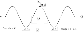
(b) Cosine function :
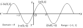
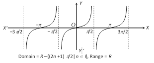
(c) Tangent function :
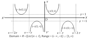
(d) Cosecant function :
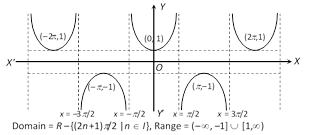
(e) Secant function :
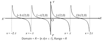
(f) Cotangent function :
(ii) Inverse trigonometric functions
| Function | Domain | Range | Definition of the function |
| \[{{\sin }^{-1}}x\] | \[[-1,\,1]\] | \[[-\pi /2,\,\,\pi /2]\] | \[y={{\sin }^{-1}}x\,\] \[\Leftrightarrow x=\sin y\] |
| \[{{\cos }^{-1}}x\] | \[[-1,\,1]\] | \[[0,\pi ]\] | \[y={{\cos }^{-1}}x\] \[\Leftrightarrow x=\cos y\] |
| \[{{\tan }^{-1}}x\] | \[(-\infty ,\,\,\infty )\] or R | \[(-\pi /2,\,\,\pi /2)\] | \[y={{\tan }^{-1}}x\] \[\Leftrightarrow x=\tan y\] |
| \[{{\cot }^{-1}}x\] | \[(-\infty ,\,\infty )\] or R | \[(0,\,\,\pi )\] | \[y={{\cot }^{-1}}x\] \[\Leftrightarrow x=\cot y\] |
| \[\text{cose}{{\text{c}}^{-1}}x\] | \[R-(-1,\,\,1)\] | \[[-\pi /2,\,\,\pi /2]-\{0\}\] | \[y=\text{cose}{{\text{c}}^{-1}}x\] \[\Leftrightarrow x=\text{cosec }y\] |
| \[{{\sec }^{-1}}x\] | \[R-(-1,\,\,1)\] | \[[0,\,\,\pi ]-[\pi /2]\] | \[y={{\sec }^{-1}}x\] |
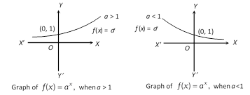
(iii) Exponential function : Let \[a\ne 1\] be a positive real number. Then \[f:R\to (0,\,\infty )\] defined by \[f(x)={{a}^{x}}\] called exponential function. Its domain is R and range is \[(0,\,\infty )\].
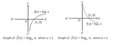
(iv) Logarithmic function : Let \[a\ne 1\]be a positive real number. Then \[f:(0,\,\infty )\to R\]defined by \[f(x)={{\log }_{a}}x\]is called logarithmic function. Its domain is \[(0,\,\infty )\]and range is R.
(8) Explicit and implicit functions : A function is said to be explicit if it can be expressed directly in terms of the independent variable. If the function can not be expressed directly in terms of the independent variable or variables, then the function is said to be implicit. e.g. \[y={{\sin }^{-1}}x+\log x\]is explicit function, while \[{{x}^{2}}+{{y}^{2}}=xy\] and \[{{x}^{3}}{{y}^{2}}={{(a-x)}^{2}}{{(b-y)}^{2}}\] are implicit functions.
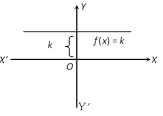
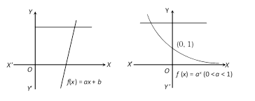
(9) Constant function : Let k be a fixed real number. Then a function f(x) given by \[f(x)=k\] for all \[x\in R\] is called a constant function. The domain of the constant function \[f(x)=k\] is the complete set of real numbers and the range of f is the singleton set \[\{k\}\]. The graph of a constant function is a straight line parallel to x-axis as shown in figure and it is above or below the x-axis according as k is positive or negative. If \[k=0,\] then the straight line coincides with x-axis.
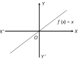
(10) Identity function : The function defined by \[f(x)=x\] for all \[x\in R\], is called the identity function on R. Clearly, the domain and range of the identity function is R.
The graph of the identity function is a straight line passing through the origin and inclined at an angle of \[{{45}^{o}}\] with positive direction of x-axis.
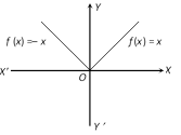
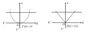
(11) Modulus function : The function defined by \[f(x)=|x|=\left\{ \begin{matrix} x,\,\,\,\text{when}\,\,\,x\ge 0 \\ -x\text{,}\,\,\text{when}\,\,\,x<\text{0} \\ \end{matrix} \right.\] is called the modulus function. The domain of the modulus function is the set R of all real numbers and the range is the set of all non-negative real numbers.
(12) Greatest integer function: Let \[f(x)=[x],\] where \[[x]\] denotes the greatest integer less than or equal to \[x\]. The domain is R and the range is \[l\]. e.g. \[[1.1]\,\,=1,\,\,[2.2]\,=2,[-0.9]=-1,\,\,[-2,\,\,1]=-3\] etc. The function \[f\] defined by \[f(x)=[x]\] for all \[x\in R\], is called the greatest integer function.
(13) Signum function : The function defined by \[f(x)=\left\{ \begin{matrix} \frac{|x|}{x},\,x\ne 0 \\ \,\,\,\,\,\,0,\,x=0 \\ \end{matrix} \right.\]or\[f(x)=\left\{ \begin{matrix} \ 1,\,\,x>0 \\ \ 0,\,\,x=0 \\ -1,\,\,x
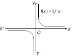
(14) Reciprocal function : The function that associates each non-zero real number \[x\] to be reciprocal \[\frac{1}{x}\] is called the reciprocal function. The domain and range of the reciprocal function are both equal to \[R-\{0\}\] i.e., the set of all non-zero real numbers. The graph is as shown.
(15) Power function : A function \[f:R\to R\] defined by, \[f(x)={{x}^{\alpha }}\], \[\alpha \in R\] is called a power function. Domain and Range of Some Standard Functions
| Function | Domain | Range |
| Polynomial function | \[R\] | \[R\] |
| Identity function \[x\] | \[R\] | \[R\] |
| Constant function \[K\] | \[R\] | \[\{K\}\] |
| Reciprocal function \[\frac{1}{x}\] | \[{{R}_{0}}\] | \[{{R}_{0}}\] |
| \[{{x}^{2}},\,|x|\] | \[R\] | \[{{R}^{+}}\cup \{0\}\] |
| \[{{x}^{3}},\,x\,|x|\] | \[R\] | |
| Signum function | \[R\] | \[\{-1,\,\,0,\,\,1\}\] |
| \[x+|x|\] | \[R\] | \[{{R}^{+}}\cup \{0\}\] |
| \[x-|x|\] | \[R\] | \[{{R}^{-}}\cup \{0\}\] |
| \[[x]\] | \[R\] | \[l\] |
| \[x-[x]\] | \[R\] | \[[0,\,\,1)\] |
| \[\sqrt{x}\] | \[[0,\,\,\infty )\] | \[[0,\,\infty ]\] |
| \[{{a}^{x}}\] | \[R\] | \[{{R}^{+}}\] |
| \[\log x\] | \[{{R}^{+}}\] | \[R\] |
| \[\sin x\] | \[R\] | \[[-1,\,\,1]\] |
| \[\cos x\] | \[R\] | \[[-1,\,\,1]\] |
| \[\tan x\] | \[R-\left\{ \pm \frac{\pi }{2},\,\,\pm \frac{3\pi }{2},\,.... \right\}\] | \[R\] |
| \[\cot x\] | \[R-\{0,\,\,\pm \pi ,\,\,\pm 2\pi ,...\}\] | \[R\] |
| \[\sec x\] | \[R-\,\left\{ \pm \frac{\pi }{2},\,\,\pm \frac{3\pi }{2},... \right\}\] | \[R-(-1,\,\,1)\] |
| \[\cos \text{ec}x\] | \[R-\left\{ 0,\,\,\pm \pi ,\,\,\pm 2\pi ,... \right\}\] | \[R-(-1,\,\,1)\] |
| \[{{\sin }^{-1}}x\] | \[[-1,\,\,1]\] | \[\left[ \frac{-\pi }{2},\,\,\frac{\pi }{2} \right]\] |
| \[{{\cos }^{-1}}x\] | \[[-1,\,\,1]\] | \[[0,\,\,\pi ]\] |
| \[{{\tan }^{-1}}x\] | \[R\] | \[\left( \frac{-\pi }{2},\,\frac{\pi }{2} \right)\] |
| \[{{\cot }^{-1}}x\] | \[R\] | \[(0,\,\,\pi )\] |
| \[{{\sec }^{-1}}x\] | \[R-(-1,\,\,1)\] | \[[0,\,\pi ]\,-\,\left\{ \frac{\pi }{2} \right\}\] |
| \[\text{cose}{{\text{c}}^{-1}}x\] | \[R-(-1,\,\,1)\] | \[\left[ -\frac{\pi }{2},\,\,\frac{\pi }{2} \right]-\{0\}\] |


You need to login to perform this action.
You will be redirected in
3 sec

